Solved

Results for high frequency approximations (Wave propagation)

  • 12 September 2021
  • 37 replies
  • 987 views

Hello,

I am a new user of the OpticStudio software which arouses my curiosity!

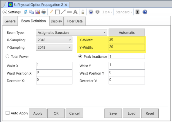
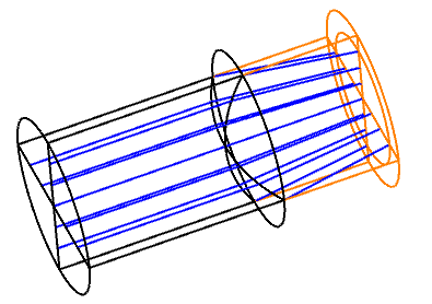
The wave propagation can be solved with several models and the software offers several possibilities. The model based on the astigmatic Gaussian beams (beamlets) is very well interesting.

But, I found few years ago the relevant paper:

Gosse L., James F., Convergence results for an inhomogeneous system arising in various high frequency approximations, Numer. Math. 90: 721–753 (2002).

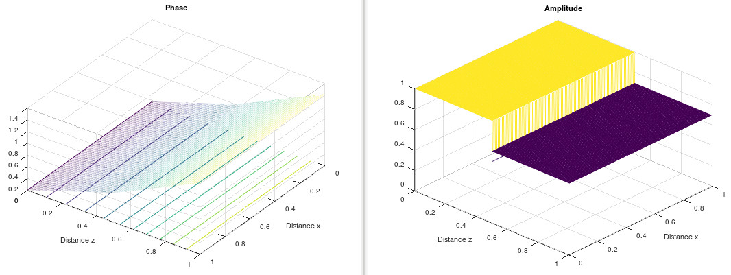
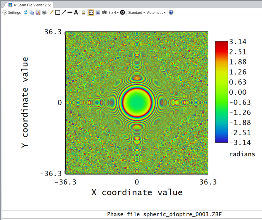
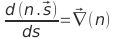
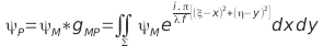
It is enough hard because the mathematics formulations are theoretic. However, the issue solving gives several possibilities to find the phase and the amplitude of the light wave together.

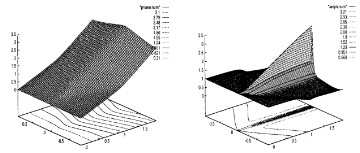
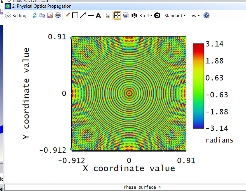
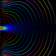
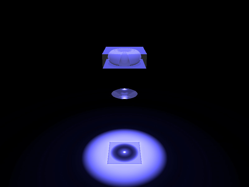
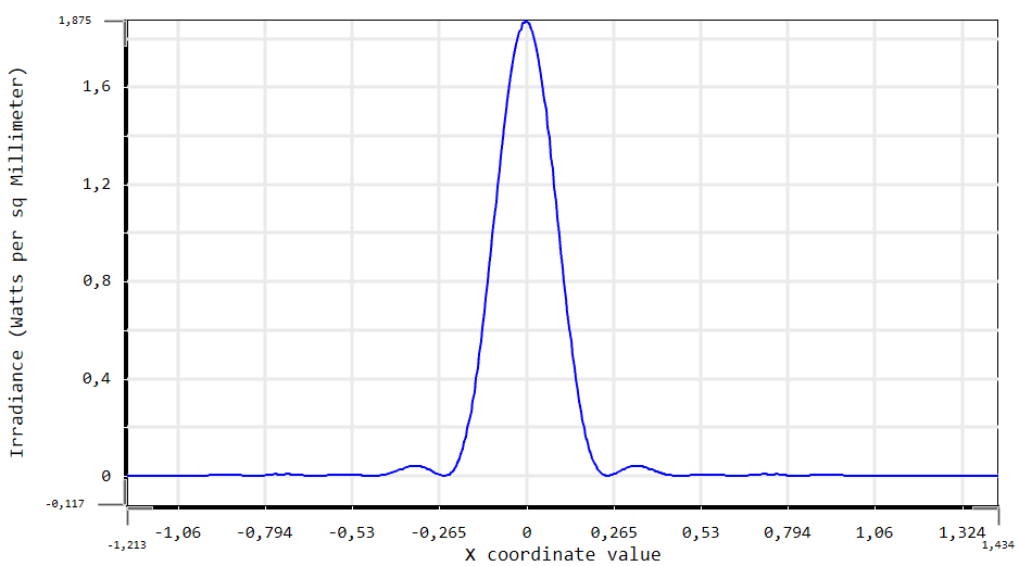
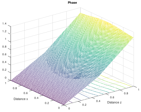
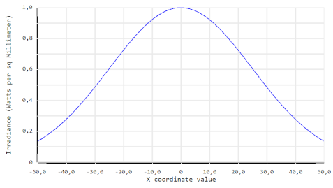
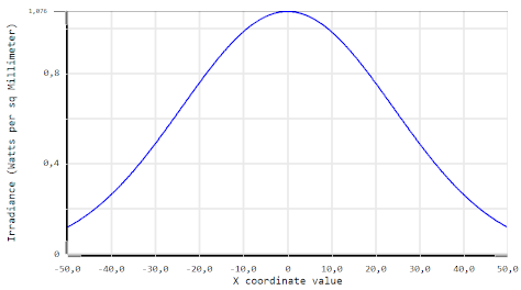
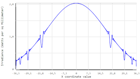
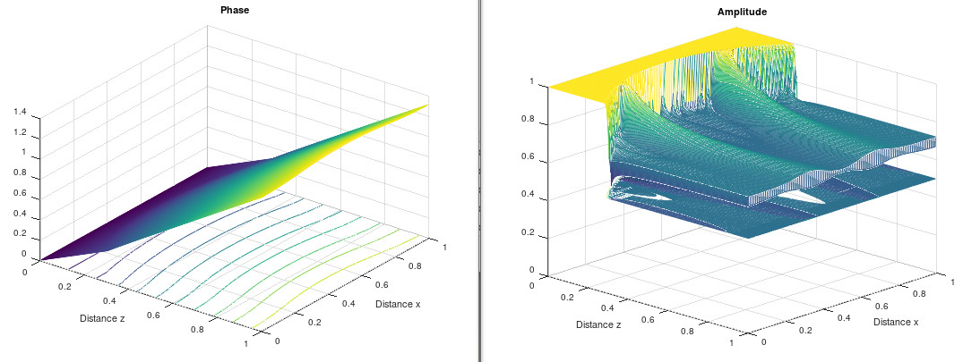
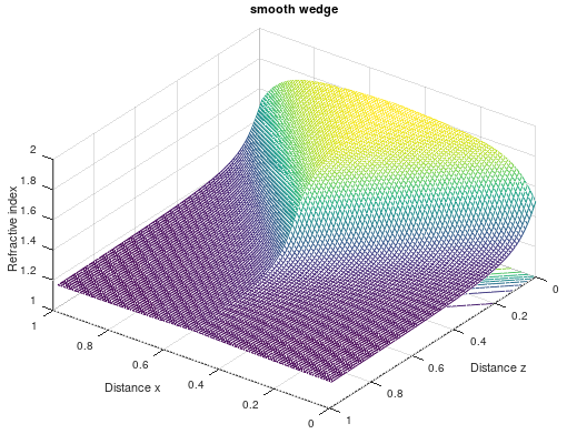
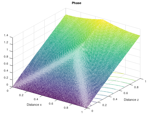
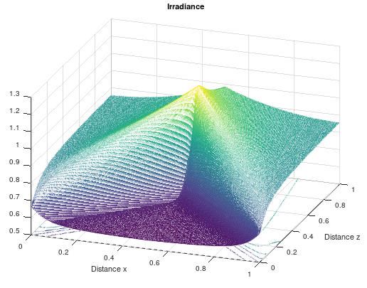
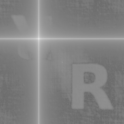
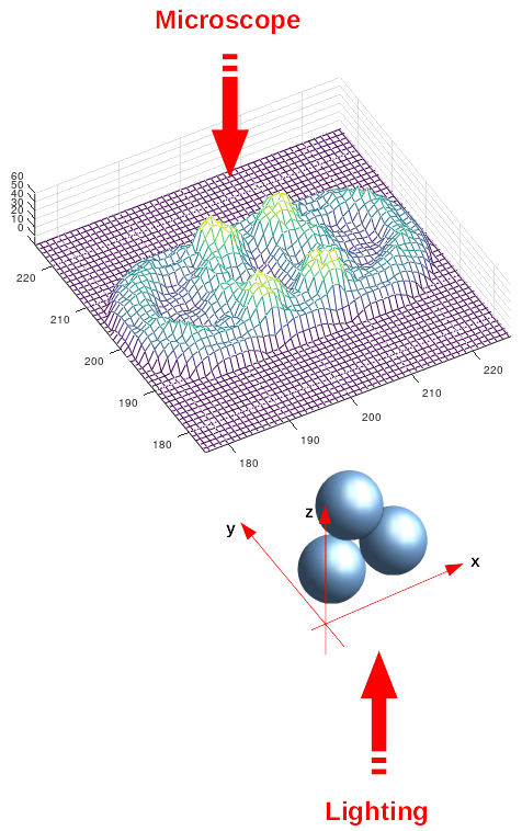
Numerical values for the phase and the amplitude of the smooth wedge.

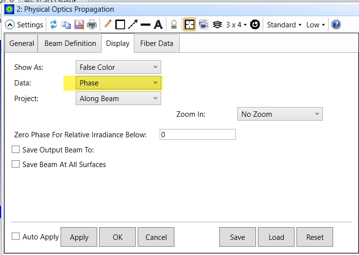
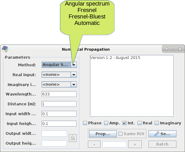
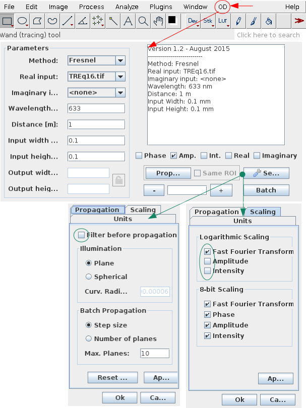
Therefore, do we have this possibility with the OpticStudio? Compute the phase in order to see transparency images for instance?

Thank you in advance for your answer.

Benoît.

icon

Best answer by Sandrine Auriol 27 September 2021, 11:30

View original

37 replies

Userlevel 4
Badge +1

Hi Plancoulaine, 

OpticStudio provides 3 methods to model beam propagation. One is based on pure geometric ray trace. You can view the phase of the beam using the Wavefront map which shows you the optical path difference of a pupil ray relative to either the chief ray or the centroid. The second is the Paraxial Gaussian or the Skew Gaussian model.  The Paraxial Gaussian computes the propagation and transformation of a rotationally symmetric Gaussian beam using two paraxial rays in a meridional plane as given by Arnaud in "Hamiltonian Theory of Beam Mode Propagation” and Siegman in “Lasers”. The Skew Gaussian can model an off-axis propagation of the beam and the beam parameters are computed using real rays and account for astigmatism. The third method is the Physical Optics Propagation (POP) where the propagation is modeled by propagating wavefronts through your optical system. The physical optics model is generally more accurate at predicting the detailed amplitude and phase structure of the beam. You can find a detailed explanation on how POP works in the help documentation at The Analyze Tab (sequential ui mode) > Laser and Fibers Group > About Physical Optics Propagation.

I’m not familiar with the paper you’ve quoted above. Could you please elaborate a bit more on what you are trying to model here? Maybe a drawing or a lens file can help. 

Best,

Hui

Hello Hui,

Thank you for your precious information.

Yes, the physic propagation module (POP) gives very good irradiance images, no problem (I tested with the knife-edge). The pure geometric ray trace with the “Jacobi-Hamiltonian” and especially the “method of characteristics” is also very good to find the light rays and the phase on the wave surfaces. I think the two modules compute independently the results but perhaps, it is not exact.

Therefore, it not is very easy to establish directly relationships between the intensity and the phase. The very simple example attached shows the Gaussian beams with the intensity superposed with the phase which are computed together. In particular, we see enough well the Rayleigh length impact on the Gaussian beams.

Kind regards, Benoît.

Userlevel 6
Badge +2

Hello Benoit

Sorry there is no attachment to your previous post. Is there supposed to be one?

Thank you.

Sandrine

Hello Sandrine,

No, I not uploaded attachment. You find attached the paper of the first message.

I began slowly the programming of the method of this paper (it is not my main activity) to study the light behaving in the biological tissues (I think it is surely interesting to have the intensity and phase image computed together).

Kind regards, Benoît.

Userlevel 6
Badge +2

Hi Benoit

Physical Optics Propagation gives both the irradiance and phase of the beam. Can this work for your case?

Sandrine

Hello Sandrine,

Yes, I found the way to simulated intensity using the “Physical Optics Propagation” module (I will surely illustrate these simulations in a future paper). Otherwise, I not found how obtain the phase, can you help me, please.

I built images from the Povray software of the biological simulations:

At the top, a nucleus for instance, in middle a lens (microscope) and at the bottom the image given by the lens.

Other biological elements without lens.

The Poveray is a good software but it is classical ray tracing. In particular, it seems to me the diffraction phenomena is lost (the photon module can reveal caustics only).

Have a good week-end, Benoît.

Userlevel 6
Badge +2

Hey Benoit!

Thank you for sharing this. It is interesting.

For the phase, I have opened the file under "{Zemax}\Samples\Physical Optics\Axicon with ring focus.ZMX". In the POP window, you can simply ask to display the phase:

The phase is atan(Imaginary part of the electric field/real part). It is between +/-π.

At each surface, we have an array containing the complex electric field so the intensity and phase are calculated from this. There is another forum post that you may find interesting here: 

Otherwise if you search for POP on our KBA website https://support.zemax.com/hc/en-us/search?utf8=%E2%9C%93&query=pop, you will get some interesting articles that I would recommend reading if you are not too familiar with POP.

Sandrine

Userlevel 6
Badge +2

And I am not sure if it can be interesting for you but we have an old article (it is not published) about a macro written to render OpticStudio lens files in POV-Ray. Let us know if this is something you’d like and I can see to send it or update it?

Hello Sandrine,

Thank you for your advises. However, I simulated circular obstruction in order to understand your propagation module.


This obstruction is built by a circular hole of 0,4 mm of diameter and it is viewed from 150 mm away.

The irradiance image and the phase image are given below (OpticStudio file is attached to this exchange).

Irradiance image

Diffraction profile

We watch the traditional diffraction profile.

Phase image

You can simulate the same issue with the “Numerical Wave Propagation” plugin by means to ImageJ software (Piedrahita-Quintero P, Castañeda R, Garcia-Sucerquia, Numerical wave propagation in ImageJ, J. Appl. Opt.; 54[21]:6410-5 (2015)). You also obtain the irradiance and phase image.

Irradiance image


Profile of the diffraction
 

Diffraction profile

We also watch the traditional diffraction profile (just a few difference scale due to the image resolution).


Phase image
 

Phase image

The “OpticStudio” simulation uses the astigmatic Gaussian beam propagation and the ImageJ plugin uses directly the Fresnel propagation. It seems to me the two phase images differ but the phase computation is perhaps different?

Yes, I am interested by your paper, thank you in advance.

I read some user guides of the OpticStudio software and I found two Zemax papers:

- Aumeyr (T.), Billing (M.G.), Bobb (L.M.), Bolzon (B.), Karataev (P.), Lefevre (T.), Mazzoni (S.), Zemax Simulations of Transition and Diffraction Radiation, J. Phys.: Conf. Ser. 517 012026 (2014).

- Ikeda (K.), Gay (S.), OpticStudio TrueFreeform TM optimization for complex illumination systems, Light-Emitting Devices, Materials, and Applications, Proceedings Vol. 11302 (2020).

Kind regards, Benoît.

Userlevel 6
Badge +2

Hi Benoit

Could you send the settings you used for POP? The easier is if you can save your file as an archive file (File...save as...zar) as it will contain everything needed.

I’ll have a look because when going through pinholes we often need to adjust the sampling for POP. There is a sample file here if you want to have a look: "{Zemax}\Samples\Physical Optics\Pinhole Aperture.ZMX".

You can see that the pilot beam is recalculated after the pinhole:
 

But sometimes the sampling needs to be changed too.

I have attached the article (sorry it is a copy and paste so the format is not great). The attachments can be found here.

Sandrine

Hi Sandrine,

Thank you for your paper, I will look it with attention.

Yes, I study the “Pinhole Aperture” but I cannot generate good results. Your aperture is defined with “Cicular Aperture” and with “Maximum radius” 0.006. I changed this last parameter but I not succeeded!

Concerning the POP parameters, I attached another zip file to this exchange, I hope it is better! But, I can give you the parameters for POP:

- Settings→ Beam: Definition: Beam Type=”Astigmatic Gaussian”; X-Sampling=Y-Sampling=2048; X-Width=Y-Width=100; Waist X=Waist Y=1.

- Settings→ Display: Show As=Inverse Grey Scale (irradiance) or Grey scale (phase) or Cross X; Data=Irradiance or Phase.

I also remake the simulation with the Numerical Propagation plugin. I improved the contrast for amplitude and I use false color this time (please, see below).

Amplitude image
Phase image
Phase image (size x 6)

In particular, the center is dark because the wave is locally plane.

Have a good weekend, Benoît.

Userlevel 6
Badge +2

Hi Benoit,

Thank you for sharing your file.

Usually, when I am working with POP, I try to set the geometric rays to be quite similar to POP. There is no really need for that but I think it helps in terms of setting the system properly.

So in POP, the waist is 1mm in radius and starts at surface 1.

In the “geometric” definition, the beam starts from surface 0 and has a divergence angle (marginal ray) of 6.3 degrees. On surface 1, the beam has a radius of roughly 24mm.

So is the POP definition correct? Does the beam start on surface 1 or does it start at the object?

Let me know and then I’ll keep on working on it.

Hi Sandrine,

Thank you for your experimentation.

Yes, I agree with you for the POP and “geometric” definitions.

The optic device is divided into two parts: 1/ planoconvex lens to build a parallel beam and 2/ a circular obstruction (radius 0.2 mm). Only, the second part is interesting for the diffraction phenomena (between surface 3 and surface 4).

Irradiance on surface 3

I study more details the Gosse’s article (first post) and I began the programming to try compare the methods. It is not finished! The final goal is to simulate the diffraction of our circular obstruction. You find a phase image of a spherical dioptre lighted by a parallel beam.

Phase image (spheric dioptre)

Otherwise, I tried the OpticStudio Macro to build a Povray file. The Povray software finds a error “Problem with option setting”. I examined the generated file and It seems to me correct? (attached with this post).

Warm regards, Benoît.

Userlevel 6
Badge +2

Hello Benoit 

I have looked at the sampling of POP in the file you attached and I have adjusted it. When going through the pinhole, the irradiance looks square because it is described by a small amount of pixels so this is what I was looking for.

So I started by changing the initial array size as the beam has a very low divergence:

Then I resampled the beam after the pinhole. The file is attached.

About the POV ray, I’ll have a look.

Userlevel 6
Badge +2

I have looked at the POV ray file but I also have an error. Different one though. I’ll check if someone internally knows how to use this.

Hello Sandrine,

Thank you, your experimentation agrees me very well.

Yesterday, I progressed the programming concerning the Cosse’s paper (first post).

Two simple tests:

First one is the plane dioptre (see the propagation of OpticStudio):

The first surface is the reference, the second surface is the dioptre (N-BK7 material) and third surface is the image.

The irradiance profile on the second surface computed with “Physical Optics”:

The irradiance profile on the third surface computed with “Physical Optics”:

The same test was performed with the Gosse’s method:

At the right, we show the irradiance (not amplitude) decreasing after the dioptre crossing due to the transmission coefficient (Fresnel’s coefficients).

Second one is the spherical dioptre (see the propagation of OpticStudio):

The first surface is the reference, the second surface is the dioptre (N-BK7 material) and third surface is the image.

The irradiance profile on the second surface computed with “Physical Optics”:

The irradiance profile on the third surface computed with “Physical Optics”:

The same test was performed with the Gosse’s method:

At the right, It seems to me we show the irradiance (not amplitude) with the caustics after the dioptre crossing.

Do you think it is possible to simulate the same effects (irradiance decreasing and caustics) with OpticStudio? What module should be to use?

The OpticStudio files are attached to this post.

Have a nice weekend, Warm regards, Benoît.

Userlevel 6
Badge +2

Hi Benoit

Sorry I haven’t read the paper yet, but are the plots you are showing along the propagation distance?

If that is the case, I suppose you could try to get similar plots using the POPI operand in ZPL or API. With the API, you can  also read the results directly. You will need to save the beam at all the Z steps you wish to have.

That being said, I am not sure that the POP results are correct as we can see that the phase sampling doesn’t look great. This is the phase sampling at surface 4 for the spheric_dioptre.zmx. We can also see that we have warnings in the Prop Report of POP:

I looked at the sampling needed in your case (see the article https://support.zemax.com/hc/en-us/articles/1500005488641-Using-Physical-Optics-Propagation-POP-Part-3-Inspecting-the-beam-phases) and I uploaded the merit function in your system and it gives me a sampling of around 16,000. 


I haven’t tried to do the calculation yet as it is quite long.

At this point I think I’ll ask one of my colleague to check because I’m not sure the software can do what you are planning to.

Hello Sandrine,

This paper is a bit hard because the authors are very good mathematicians. I unscrambled few demonstrations for the programming of their method in 2D which diverges for some cases but which expands to the 3D. I therefore retain only the first paragraphs and the figures. I remade nearly their figures (see below by centring the smooth wedge and taking "z" as optical axis).

Their optical component
The phase image of the smooth wedge
The irradiance image of the smooth wedge

Tomorrow, I will study the POPI operand in ZPL and API. I not known yet these operands. I should have surely few questions!

Your beautiful phase image seems to me correct because I find again there bubble clusters due to phase computations, thank you.

Warm regards, Benoît.

Userlevel 6
Badge +2

Hi Benoit,

Please allow me to reply as I have also checked this discussion.

I have a few comments to what have been discussed so far.

  1. About the method used in Zemax OpticStudio, it’s mainly a mix of the so-called Fresnel propagation and the Angular spectrum propagation. The method in ImageJ based on FFT can be also considered as Fraunhofer propagation. Fraunhofer propagation is the simplified version of the Fresnel propagation. Fraunhofer propagation only works when the beam is propagated to far field or when it’s focused by a lens. I think the Physical Optics Propagation (POP) in Zemax OpticStudio should be more accurate when it’s far from the above cases. If you are interested in knowing more details of Fresnel and Fraunhofer diffractions, you can refer to the book Introduction to Fourier Optics by Goodman.
  2. As far as I know, POV rays is based on pure geometric method. It doesn’t provide phase data and even the coherent intensity data. I think it’s hard to compare its result with POP.
  3. About the example file you provided in spheric_dioptre.zar, I agree with Sandrine that this is too challenging for Physical Optics Propagation of ZOS. The main problem is the lens you build in the system is with too high curvature that introduces very large phase slope. Those what you called bubbles are aliasing. There are severe aliasing in the phase profile. This basically means any propagation result after this surface is not trustable. The only method to solve this issue is to increase the beam sampling. I have tested beam sampling with 16384x16384, but have no luck. Unfortunately, I think the conclusion is you cannot use POP with this highly curved lens. If you mainly want to compare the result in POP with your code, I suggest you try a milder curvature for your lens.


Please let me know if you have any more questions.

Thank you!

Hi Michael and Sandrine,

Thank you very much for yours answers.

1. The “numerical propagation” plugin of the imageJ software is able to use the “angular spectrum propagation” and/or “Fresnel propagation”.

Numerical propagation module

Ours students work with this plugin to simulate the Fresnel’s holograms, for instance:

Hologram of the “R” char

I not used yet OpticStudio for the holograms, I am a Zemax beginner! Surely, OpticStudio is better and I will study your tool to propose new exercises for the students. Your OpticStudio tool is very well!

2. I agree for you. I not know perfectly your tool but I think it are two independent modules.

The POV module is surely based on the common Descartes’ law (see below in Frenet’s dynamic coordinate system)

Common Descates’ law

Therefore, only the light rays taken account.

The POP module is based on the wave propagation (angular spectrum, Fresnel) but I think you must also take account the paraxial assumption (required for FFT) . For example for the Fresnel formula, the convolution formula must be used (see below with scalar electric field “psi”).

Fresnel’s convolution formula (linear systems)

3. Thank you for your experimentation, it is interesting. I wish also to test OpticStudio for my research work concerning the histological imaging. The goal is to understand how the image training by the biological specimen. Perhaps, the Gosse's paper could give a answer because it seems to me it is possible to compute a image from several intensity plans inside of specimens. The advantage of this method is that the computations of the phase and the irradiance perform together without the paraxial assumption.

Have a nice day, Benoît.

Userlevel 6
Badge +2

Thank you Benoit. I didn’t know about that plugin. I have copied the link here if anyone is interested: https://unal-optodigital.github.io/NumericalPropagation/.

Hello Sandrine,

Just a small demo in images.

When you run imageJ with the “numerical plugin” (version 1 or 2), you can run this plugin as below:

ImageJ with the plugin

From a image of the equilateral triangle:

Source image

You obtain:

Result image after the propagation (1m)

the irradiance image with the colormap named “red hot”.

Thank you Sandrine,

Benoît.

PS. I attached a ZIP file with the images.

Userlevel 6
Badge +2

Hi Benoît,

Thank you for sharing the information!

  1. The plugin is very interesting. Although it still depends on the implementation, but I agree then this plugin is at same accuracy to POP in theoretical level, at least for simple propagation.
  2. I didn’t know into this details and thank you for sharing the theory behind the POV rays! I think you are correct that Fresnel has some paraxial approximation. Angular spectrum in theory doesn’t have paraxial approximation, but it’s only numerically applicable if the beam is not too diverging.
    1. Note all these are limited to scalar diffraction assumption. It’s correct if we only propagate the beam in free space (homogeneous and isotropic). When the beam passes through a boundary of AIR/Glass like with a lens, the probing rays are used to transfer the beam from “this side” to the “other side”. To this point, the Goose’s method looks interesting and thank you for sharing again.
  3. I don’t know Goose’s method very well, but it looks to me it’s a strength if it can handle for highly curved surface very well, although I wonder if there is any drawback on the other hand.

Thank you!

Michael

Hi Michael and Sandrine,

Thank you very much for your interesting comments.

1. The ImageJ plugin exploits the Fresnel’s propagation only from images. I think OpticStudio is able to simulate this propagation through optical device, it is a main difference. But I yet must work to adapt exercises for the students. Another analysis is the “metaxial approximation” theory by Georges Bonnet and Pierre Pellat-Finet in order to move away a bit of the “paraxial approximation” (based on the signal processing).

2. It seems to me the angular spectrum algorithm is based on the Fourier basis and uses when the distance with the source is small (the mode “automatic” of the ImageJ plugin takes account this distance in order to switch between "angular spectrum" and "Fresnel propagation").

3. Even if I know the optical equations since a few years ago, the Gosse’s algorithm is also new for me. I programmed the base of this algorithm in C language and I use “Octave software” (version freeware of Matlab) and a bit ImageJ for the illustrations. This prototype is not yet very robust because I not taken fully into account the numerical divergences. It is exactly the Gosse’s work in his paper. Nevertheless, this way seems to me promising and I hope write a simple letter in a journal to show the power of this algorithm. Unfortunately, this paper type (between practice and theory) is not very easy to publish.

Our issue is to understand the path of light through samples (see below, please)

Three water bubbles in the space whose the centers are arranged in an equilateral triangle.

Three water bubbles in the space whose the centres are arranged in an equilateral triangle.

It is the last simulation of a image stack by means of the Gosse’s prototype.

Warm regards, Benoît.

Userlevel 6
Badge +2

Hi Benoit,

I’m very sorry for late reply.

  1. Thank you for sharing again. That is a lot of information to me. I think what you mentioned is that introduced in this paper. I had read a little but obviously I need more time to understand it. The change of plane based field to spherical based is interesting. In POP, we also reference the phase to a sphere in order to decrease required grid sampling rate, but I think they are totally different technique.
  2. I would say the Angular Spectrum propagator is mainly good in any case where the beam size doesn’t change too much before and after the propagation. At least it is so in POP’s implementation. For a Gaussian beam, this means it’s only applicable for the beam propagation inside of the Rayleigh range. When the beam start or end at outside of the Rayleigh range, POP will switch to use Fresnel propagator.
  3. The use case you showed is definitely something that POP cannot handle. POP mainly considers the case of beams not too diverging and the lens curvature not too large. Some small particles (water bubble) are something POP’s algorithm cannot handle for now unfortunately. It’s amazing you can you combine these tools and make the prototype. I hope one day we could have this kind of feature to support your case. If you didn’t show me Goose’s method, I would say this kind of structure might require FDTD or BPM, but I might be wrong. One thing I noticed is that it looks like Goose’s method is based on scalar diffraction.  If the water bubble is too small, I wonder if it becomes important to consider vector diffraction.

Thank you for the information and sharing your works again. I’m sorry that I feel POP may not be very useful in some part of your system, but please let me know if you have any questions to the method we used in POP!


Best regards,

Michael

Reply