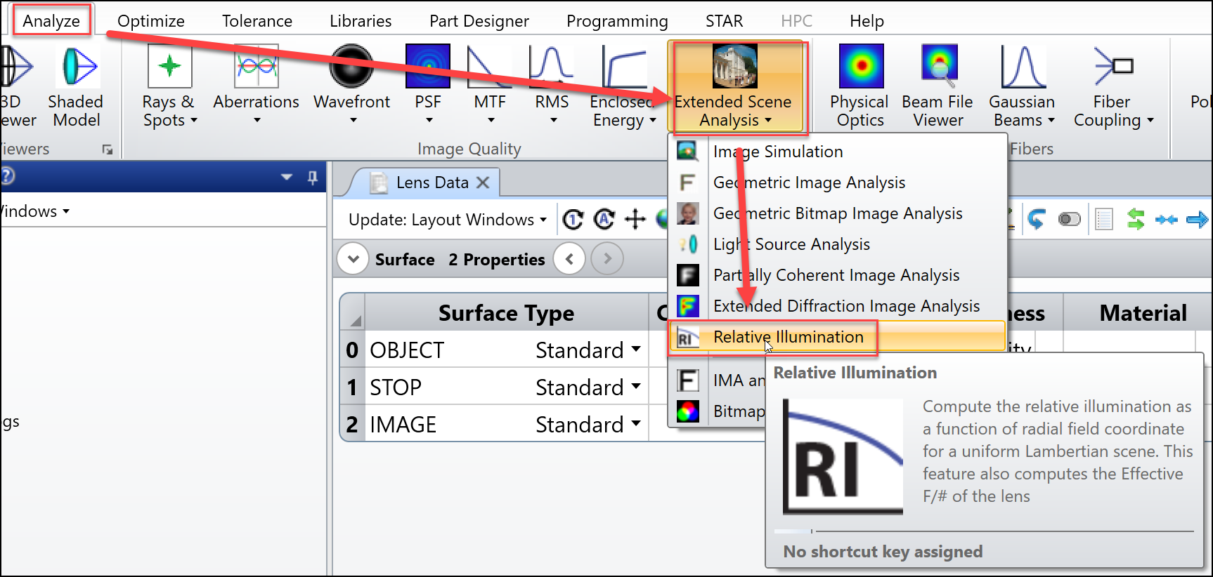
Sometimes, we may design the system starting from the 'image' back to the 'object'. For example, this is often the case for those systems that are designed to be viewed by eye, like AR/VR, HUD. In this case, normally, if we want to check the relative illumination, we need to reverse the system to check because the tool 'Relative Illumination' only calculates that on last surface in the system.

Here we will provide another way to calculate it using a macro so that you don't need to reverse the system.

Note here we at the same time is also demoing how you can verify the calculation theory of the RI. RI is actually much easier to calculate if the system is reversely designed!

First, by reading the following forum post, we know that relative illumination at each field is exactly linearly dependent to the area of the beam in cosine space in image space.

So, here is the plan. We want to write a macro to calculate the beam area in cosine space for each field, normalize it, and then get the the RI.

For simplicity, we assume the system only has apertures but no obscuration. Also we assume the chief is able to pass the system without vignetted by apertures. Note but we do will consider the effect of vignetting by aperture. In other words, if this a traditional rotationally-symmetric lens, this macro should work well.

Let's first demo how it works and then explain the code.

1. Open the \Documents\Zemax\Samples\Sequential\Objectives\Cooke 40 degree field.zmx

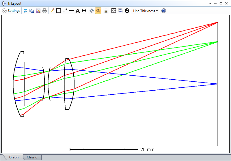
2. Turn on Ray-Aiming

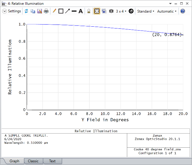
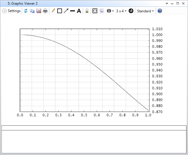
3. Open the RI with default setting and check the result as below.

4. Remove all solves on Radius and Thickness.

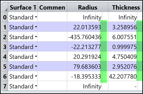
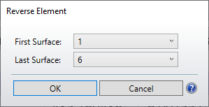
5. Reverse the system from surface 1 to surface 6.

6. Copy the thickness from last one to first.

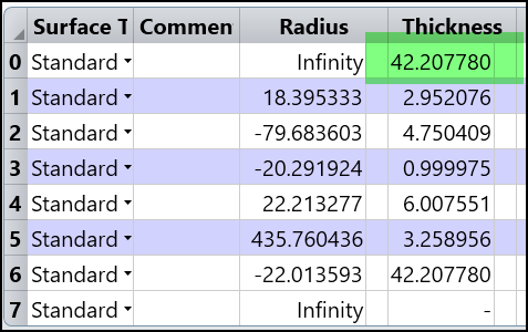
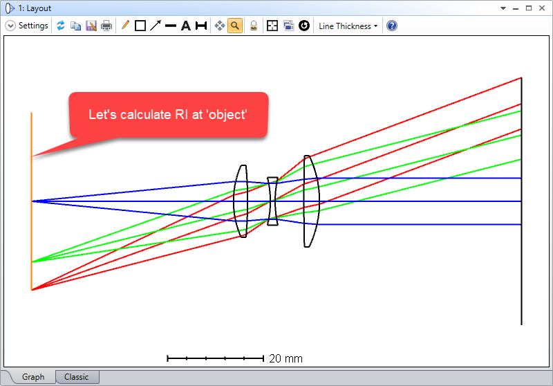
7. Now run the attached macro and we can see the result is same as the RI we calculated before reversing the system!

Now, let's check the code.

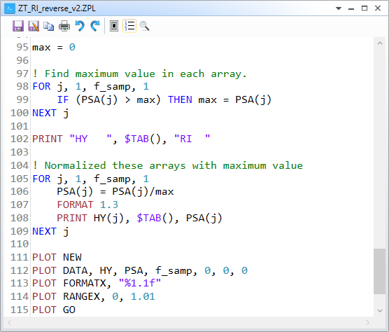
1. At first, we mainly set two variables for sampling rate and two array for saving the data to plot later.

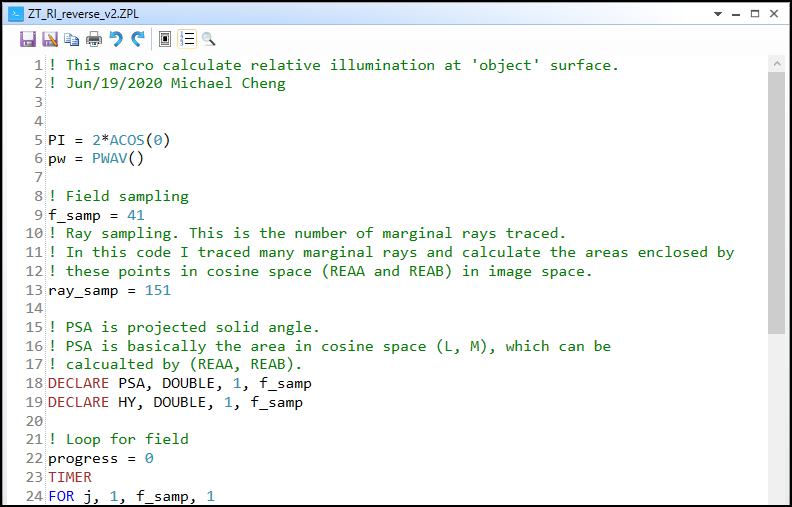
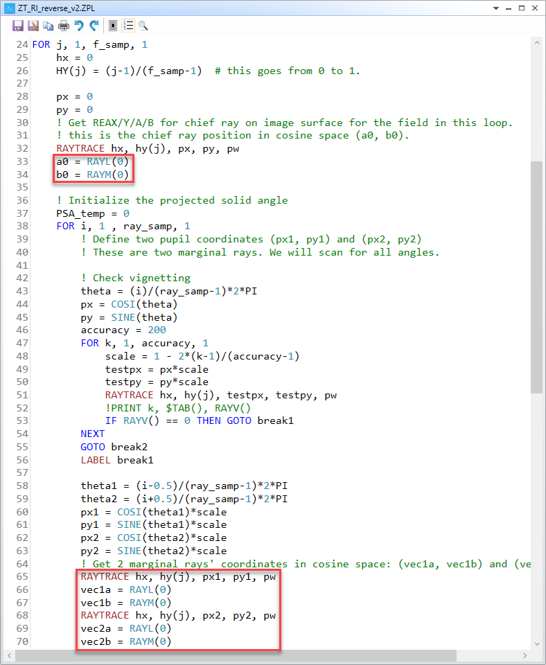
2. In the loop, it will be easier to start from looking at the 3 set of coordinates that is in cosine space. (a0,b0), (vec1a,vec1b), and (vec2a,vec2b).

Note there is one special part in line 46-54. At this part, we are check if there is any vignetting in the system. The loop first check the marginal ray which has px^2+py^2 = 1. If this ray is blocked by aperture, RAYV() will return non-zero. Then we trace another moer 'inner' ray by a scale. This loop test the scale from 1 until -1 and stop when it finds the ray can pass. By doing this, we can know the correct cosine space area considering the system apertures.

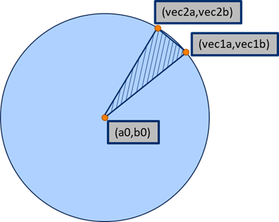
These three points are in the cosine space. The (a0,b0) is of the chief ray. The other two points are of the marginal rays. The idea is that we can use the highly sampled polygon to estimate this beam's area in the cosine space. We just need to loop for all the triangles as shown below and sum up their area.

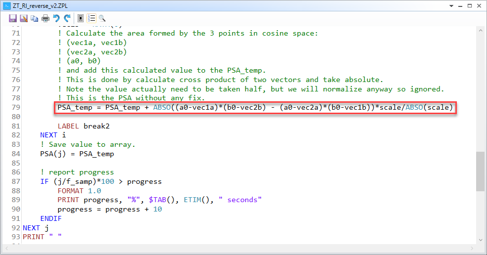
3. It can be seen how we calculate the area of the triangle and accumulate the total area at line 79.

4. Finally, at line 97-109, we simply normalize the series of the cosine space area by its maximum. Then we plot it in line 111-115.