This is a good question that we see from time to time. The Detector Polar object is physically defined by its angular characteristics, so if you have a point source at the very center of its curvature, it will exactly intercept a cone of rays if the Maximum Angle of the detector matches the Cone Angle of the source, but rays can intersect the detector that are not recorded if you are using other geometries. This is best shown with a couple of extreme examples, which are included in the attached zipped file.

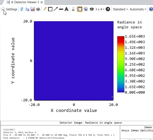
First, you can have a beam with low angular spread that completely fills the detector but shows only a narrow spot in the middle of the detector. This is the situation shown below from NarrowBeamWideDetector.zos.

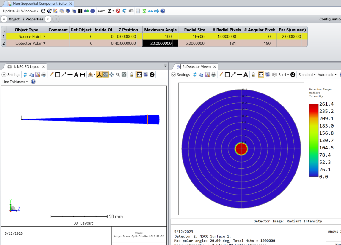
A beam with a two degree spread nearly fills a detector with a twenty degree maximum angle. Appropriately, it shows us as a narrow spot. If you bring the detector in closer, the spot display will be unchanged even though it is physically smaller.

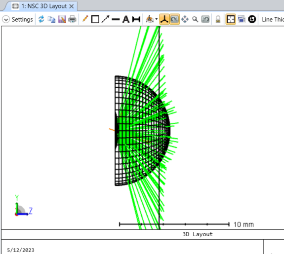
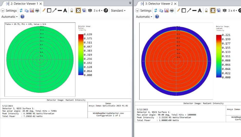
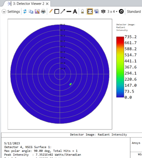
The opposite case is usually a little harder to intuit. The test case, in WideBeamNarrowDetector, has a very wide beam intersecting two Detector Polar objects, one set to 20 degrees and one set to 90. By the geometry, all rays physically go through each polar detector, but a ray trace will reveal that while the 90 degree detector records a million hits, the 20 degree case only records a bit less than 73,000 hits, with corresponding reduction in total power. This does not meant that the ray ignores the detector entirely. Applying an ABSORB material on the smaller detector will block all rays entirely. The plots are shown below.

An additional issue can arise if we view the Directivity plot option. Even with some smoothing, we see an interesting rippling in the middle, at the low angles.

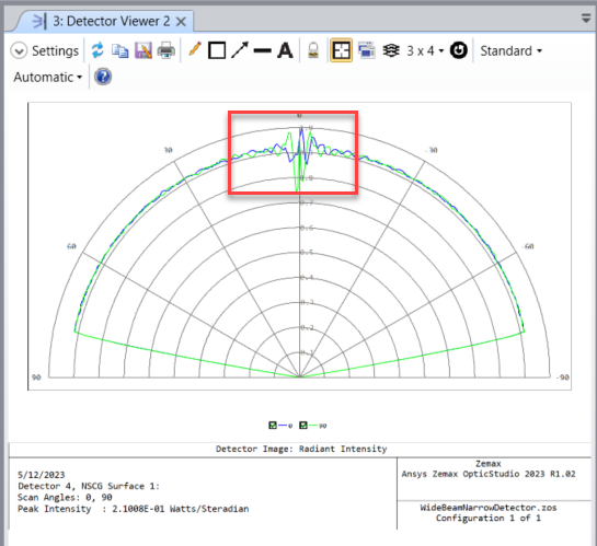
This is normal, and is analogous to the situation with position space plots. The pixel size, in the latter case, determines the resolution of the position space detector output, and a coarse sampling leads to a coarse plot. A similar thing is happening here because in polar space, the pixels close to the center axis are physically smaller than for larger angles. This may be counterintuitive, in that the low-angle ray may physically intersect the detector some distance from the center as we saw in the previous case. The pixels seem to correspond to the wire-grid display shown on the NSC 3D Layout plot. So remember that lower angles are sampled more finely by the math of polar coordinates, so there is inherently a bit more noise in the very middle of the plot, which can be removed by increasing the ray count or applying some smoothing to the data.

The final question here is about the Detector Rectangle object and the Detector Viewer displaying angle-space data. We can limit the angular resolution using the parameters X Angle Min, X Angle Max, Y Angle Min, and Y Angle Max cells, which in the example included are set to 20 each. The graph looks filled much as in the 20 degree Detector Polar case, but with almost 93000 hits rather than 73000.

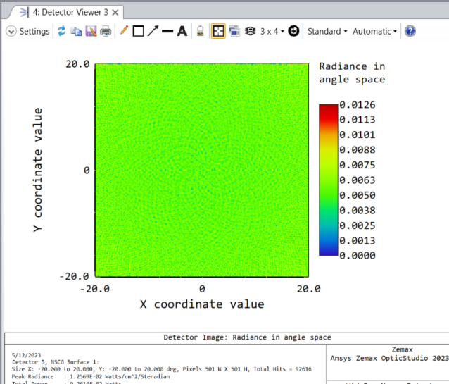
This is the main difference between the rectangular and polar cases, in that the rectangular geometry allows for spots in the corners that are within 20 degrees in each of X and Y individually, but more than 20 radially. The sample has a second Source Point with X and Y tilts set to 19 each. If we set that source to 1 ray and the other source to 0 rays, we can isolate this effect. The narrower Detector Polar shows no hits, but the larger shows a single hit at almost 30 degrees, and similarly a single spot appears in the Detector Rectangle.

So in the end, remember that the Detector Polar is both defining a region of space in which to record rays and simultaneously setting the parameters for which rays to record, and rays that hit it may be ignored for purposes of data recording, while still being noticed for other effects like MIRROR or ABSORB material properties. This is unlike the case in the Detector Rectangle where the user may specify Front Only and will completely ignore rays hitting from behind, including material properties.

The Detector Polar should be placed to capture all rays of interest, even if it does not appear to be perfectly symmetric with a perceived center of the source rays. Wide angle rays do not need to be anywhere near the outer physical pixels to be recorded as long as they are within the range set.