Solved

Quantifying straylight effect on MTF


Hi,

we are doing non-sequential simulations of surface roughness scatter, and would like to find a way to translate those into loss of contrast.

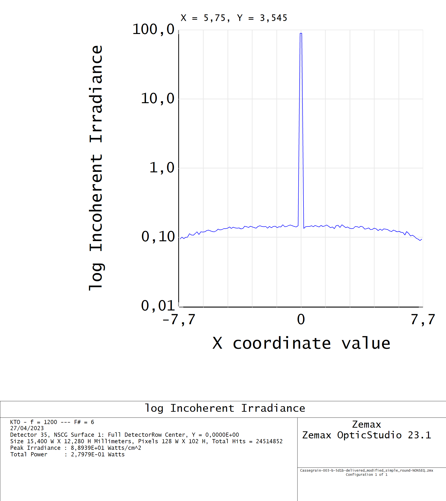
As an example, this is the type of irradiance profile we would get:


If you change the detector viewer to “Geometric MTF” you get this:


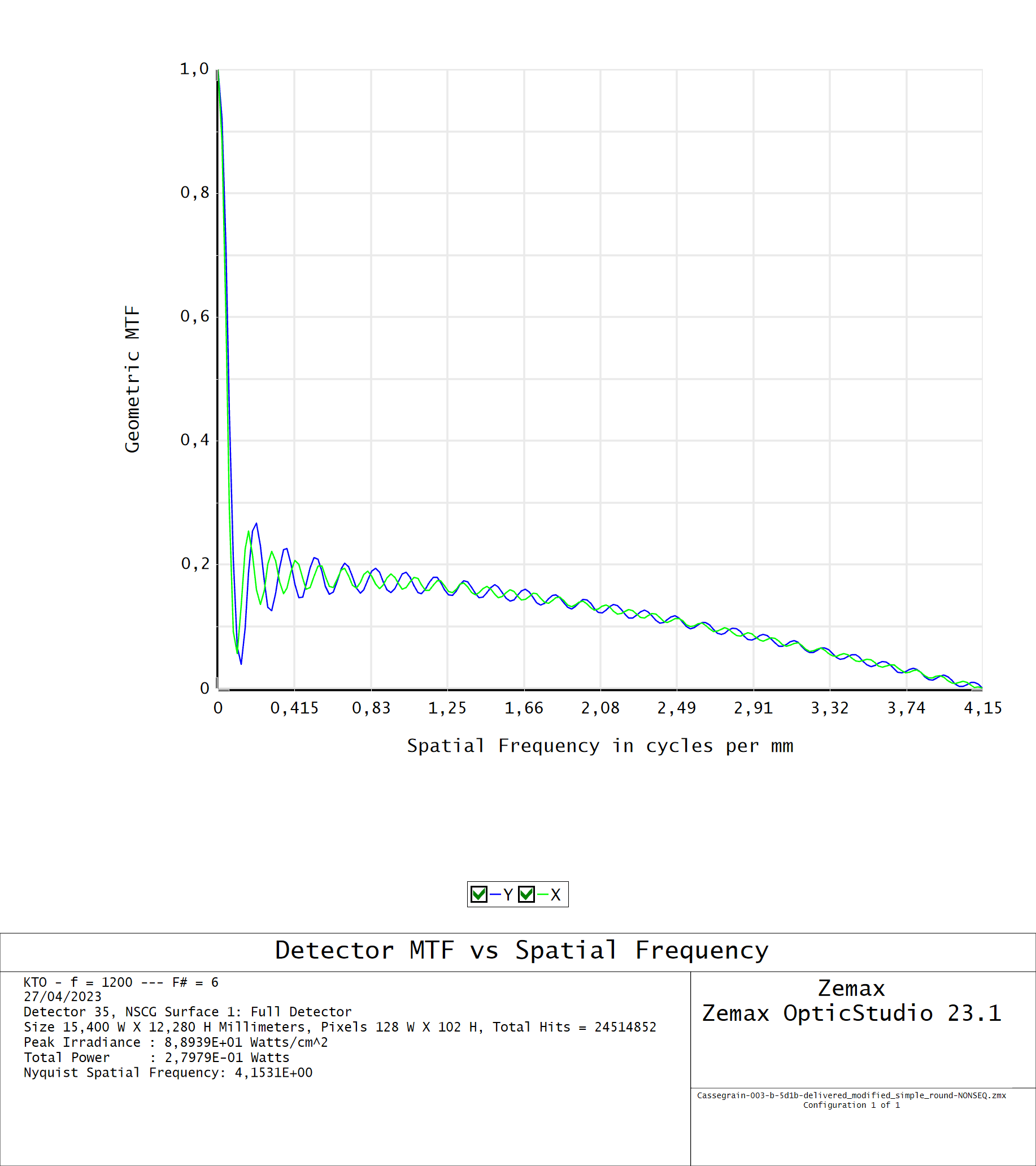
Which if I understand properly would be the Fourier transform of the “irradiance PSF”. The fact that the graph ends at 4.15 cyc/mm is because we are using pixels 10 times larger than the real detector to get enough SNR, so it’s a ten times smaller Nyquist frequency. But I don’t really know how to get any useful information on the loss of contrast from veiling glare in the image from this figure, if that is even possible.

Thanks in advance,

Alba


icon

Best answer by Mike.Jones 3 May 2023, 17:02

View original

12 replies

Userlevel 7
Badge +3

Hey Alba, haven’t you answered your own question? You need to increase the resolution of the detector.

Dear Mark,

thanks for your reply. Increasing the resolution of the detector changes the scale of the axis but does not change the overall shape of the plot, which is what I do not understand. I do not understand why it drops so quickly, and how this relates to the actual (diffraction included) MTF of the system. Overall, my goal would be to check how the surface scattering affects the system MTF.

Thanks,

Alba

Userlevel 7
Badge +3

Hey Alba,

Contrast is (Imax-Imin)/(Imax+Imin) as a function of spatial frequency.

Imagine stray light that was a constant background level. That will reduce the contrast because Imin will increase everywhere. Now give the stray light some structure, so it’s brighter in some places than others. Imin will now have a spatial frequency component that interferes with the regular MTF. I don’t think there is any analytic way to examine the structure, so OS simply ‘takes what it’s given’ and computes the MTF with whatever the light distribution is.

Does that help? I don’t feel like I have answered the question “I don’t really know how to get any useful information on the loss of contrast from veiling glare in the image from this figure” other than to play with it and see. You could save a ZRD of the direct, intended signal and save a ZRD of the stray, and then add them together in varying ratios and see the effect of the stray on MTF as you turn up the intensity of the stray light.

Hope that helps, but please continue the discussion. I think its a really interesting topic

  • Mark
Userlevel 5
Badge +3

If not too severe or spatially large (such as ground glass), scattering simply multiplies the MTF by a constant across all spatial frequencies except at f=0, where the MTF must be 1.0 as it is an autocorrelation.  The constant can be approximated by using the total integrated scatter (TIS), calculated as TIS=(4πS/wavelength)², where S is the RMS surface roughness in the same units as wavelength.  The MTF multiplier is then 1 - TIS.  For example: if S = 100Å and the wavelength is 5500Å, S=0.052.  The MTF values with zero scattering are all multiplied by (1 - 0.052) or 0.948, except at f=0, where the MTF must remain at 1.0.

Userlevel 7
Badge +3

Thanks Mike! But just to be clear, that assumes the stray light is a constant over the detector, right?

Userlevel 5
Badge +3

Yes, uniform over the detector, and possibly the entire FOV.

One note: for mirrors the TIS formula is (2πS/wavelength)².

Userlevel 7
Badge +3

You guys may also want to take a look at the book Statistical Optics, 2nd Ed. by Goodman -- specifically, Chapter 8 (Imaging through Randomly Inhomogeneous Media), Section 8.1 (Effects of Thin Random Screens on Image Quality).  Not that a thin scattering screen is the best model for veiling glare in a lens system, but the analysis does lay a basic foundation that could be used for testing a first-pass model in OpticStudio before extending the model to the veiling glare case. 

I’ll see if I can distill the salient points here.  First, the geometry of the problem is illustrated below, with the scattering surface located in the pupil of the imaging system:


Goodman begins by showing that the OTF for this case is given by a product of the OTF for the ideal imaging system times an OTF that captures the impact of the random screen:


Of most interest is a random phase-only screen:


Assume the phase at any (x,y) location is a Gaussian random variable, with the “strength” of the scattering being characterized by the phase variance.

Plugging 8.2-1 into 8.1-8, and going through some statistical analysis, Goodman shows how the autocorrelation function of the screen (8.1-8), and hence the OTF of the screen, depends on both the phase variance (which is just a number) and the normalized autocorrelation function of the random phase distribution.  The result is:


That’s the math part.  Here are some example results. 

Therefore, we see that the imaging system OTF in the presence of scattering is reduced by a multiplicative function (i.e., the OTF of the screen) that can dramatically suppress higher spatial frequencies, with the effect becoming more pronounced as the phase variance increases (i.e., as the degree of scattering goes up). 

The PSF is the inverse Fourier transform of the system OTF.  Here are some example PSFs:


Sorry if you think I’ve gone a little too far into the weeds, but this is an interesting application of statistical optics.  It would be cool if similar results could be obtained with a model in OpticStudio.

Regards,

Jeff

Userlevel 7
Badge +3

PS: When the random phase distribution of the screen is extremely fine-grain, then it’s reasonable to approximate the phase autocorrelation function as being one at the origin and zero otherwise (i.e., analogous to spatial white noise).  In this case, the OTF of the screen can be simplified:

and if the scattering is very weak, such that the phase variance is substantially smaller than one, then further simplification yields:

which agrees with the result that Mike stated in his post above.

Userlevel 5
Badge +3

Thanks, Jeff.  So to answer Pablo's original post, if the RMS surface roughness is known, and the pixel size is known, he can write a simple macro to multiply the optical system MTF by the (1-TIS) constant and the sampling MTF = sin(πfw)/(πfw) where f=spatial frequency in cy/mm and w=detector width in millimeters.

Userlevel 7
Badge +3

Wow...what a thread!

Userlevel 6
Badge +2

And if we’re already writing scripts, to account for diffraction, you can turn on the Huygens PSF flag, get the diffraction PSF, take the FFT and get the diffraction optical MTF.  

It would be nice if non-sequential mode had an option to define an F/# for multiplying the Geometric MTF by the diffraction limit (to align it with the sequential Geometric MTF) and to provide the Huygens MTF if the Huygens PSF is already calculated.

Userlevel 7
Badge +3

Mike:

Without knowing anything about the optical path (whether the dominant veiling glare is coming from multiple spurious Fresnel reflections, scattering from the optical surfaces, and/or scattering from the mechanical mounts) it’s hard to known whether or not your proposed approach is sufficient to capture MTF degradation.  However, if we can *assume* the glare is essentially due to scattering that is coming predominantly from one optical surface, and the surface roughness is small-amplitude (with a known rms) and fine-grain (very narrow autocorrelation function), then the scattering should be weak and very broad in angle, so your approach should provide a reasonable estimate for contrast reduction.

As far as including the MTF associated with a pixelated sensor, that would be good if the number of pixels sampling the primary peak of the PSF is small (say 3x3 or 4x4).  However, if the sampling is greater than that, it’s probably okay to neglect this contribution.

Regards,

Jeff

Reply