Question

New Exit Pupil Drawing


Userlevel 7
Badge +3

Hey Zemax team,

Sadly my license for OS does not include the new ‘draw entrance and exit pupils’ feature, but I saw a posting on LinkedIn that leads me to think it’s not correct. https://www.linkedin.com/posts/ir-ekim-yildirim-bb9481161_did-you-know-that-zemax-2024-r1-can-draw-activity-7179440511521292288-86_4?utm_source=share&utm_medium=member_desktop

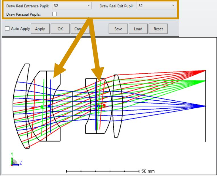
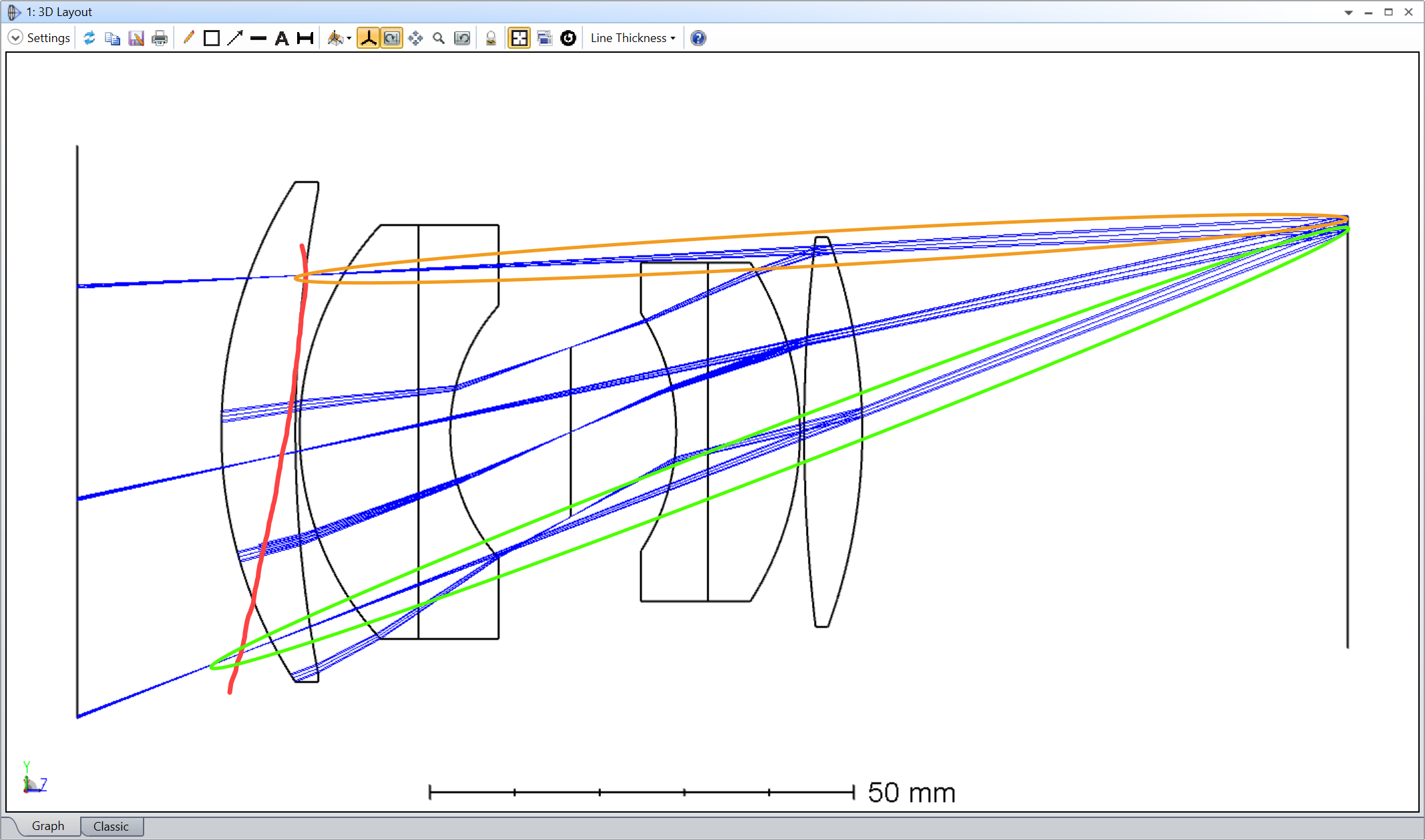
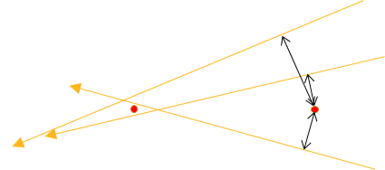
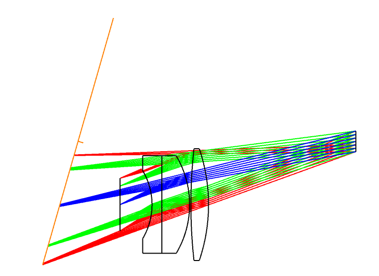
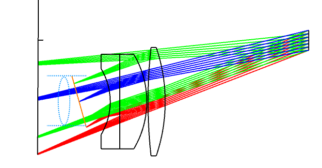
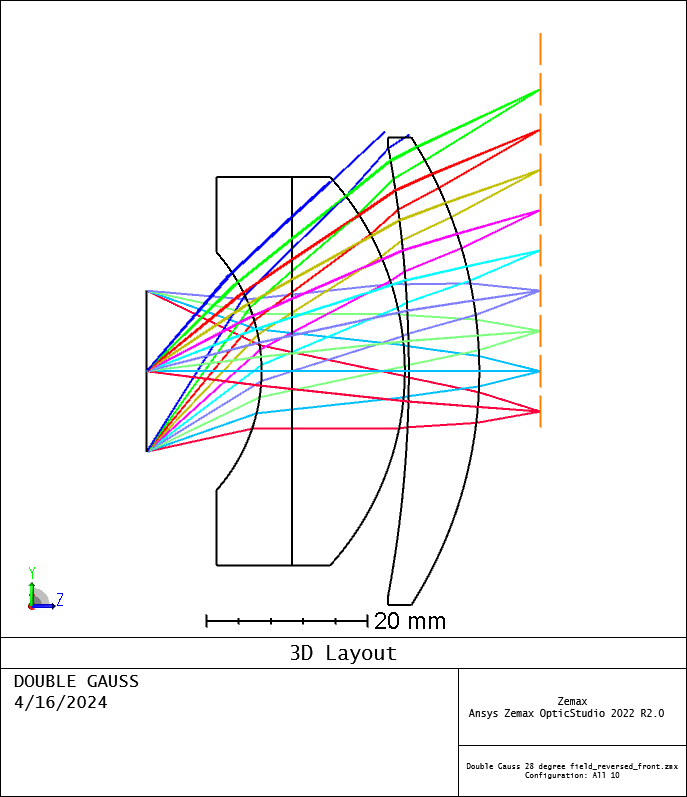
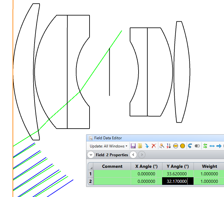
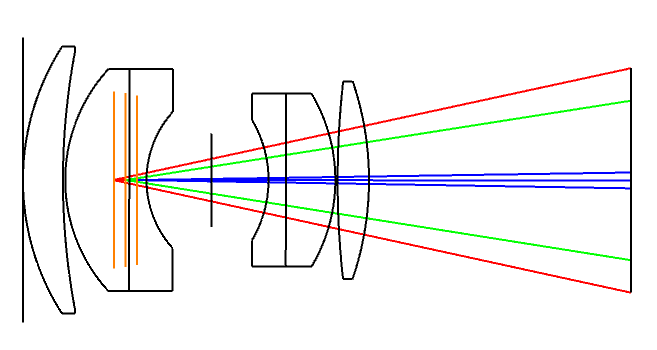
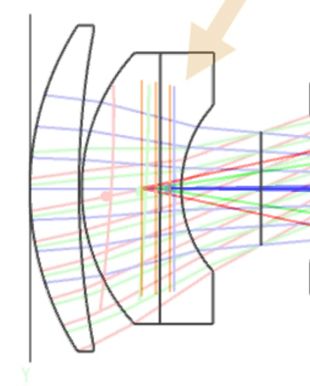
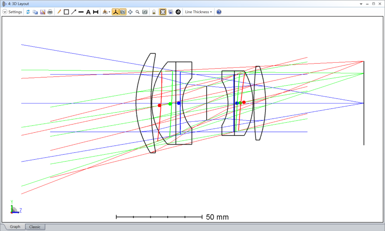
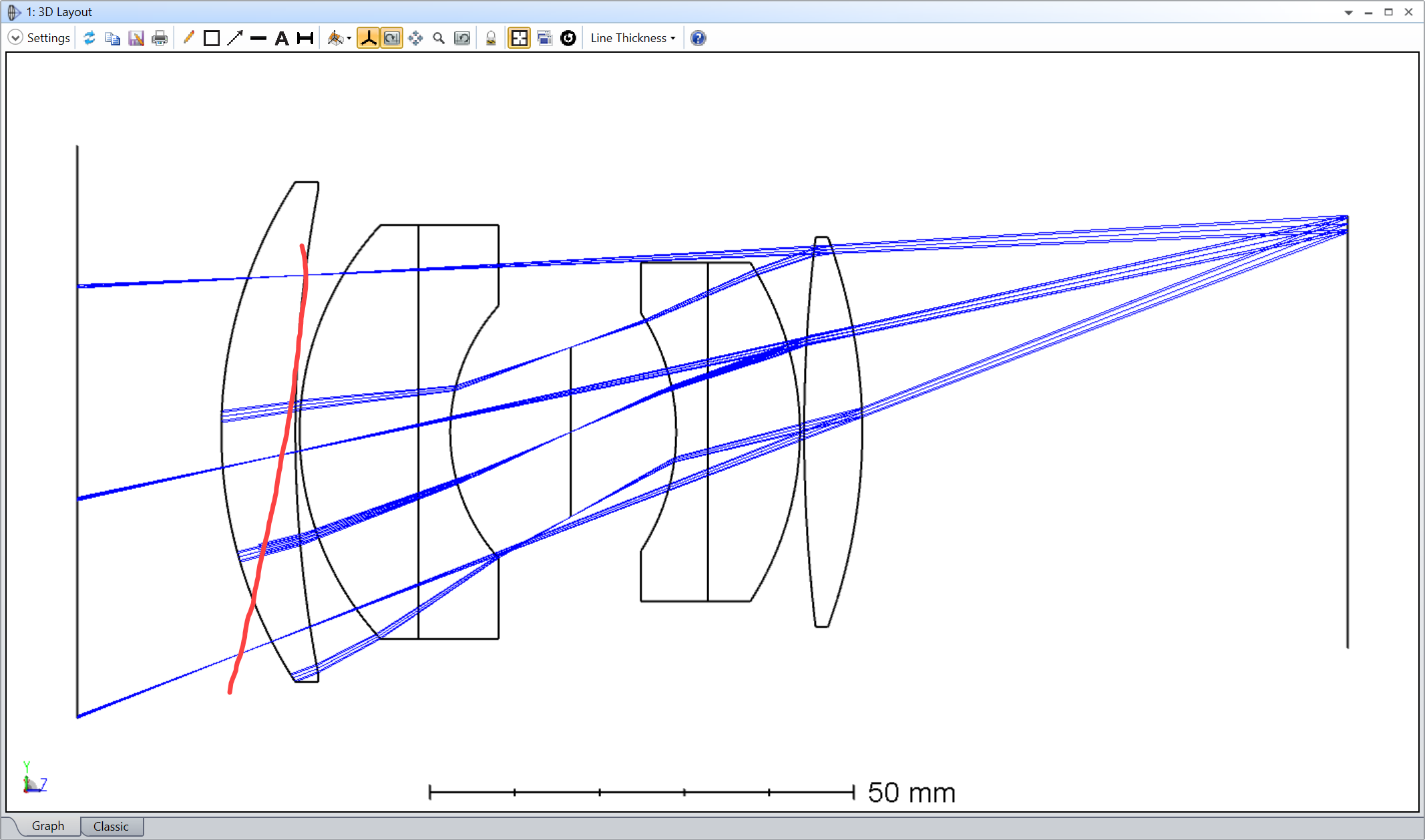
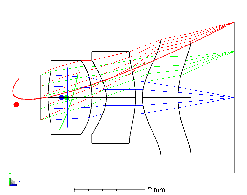
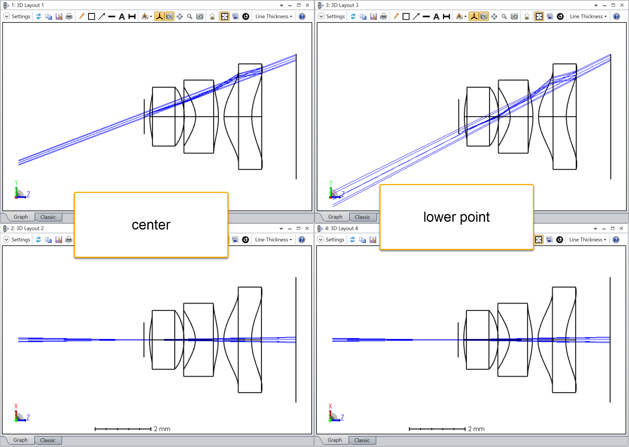
I’m assuming that the red pupils are the off-axis pupil (and so sees the red rays). The pupils appear to me to be:

  • tilting the wrong way
  • not centered on the chief ray of the field point

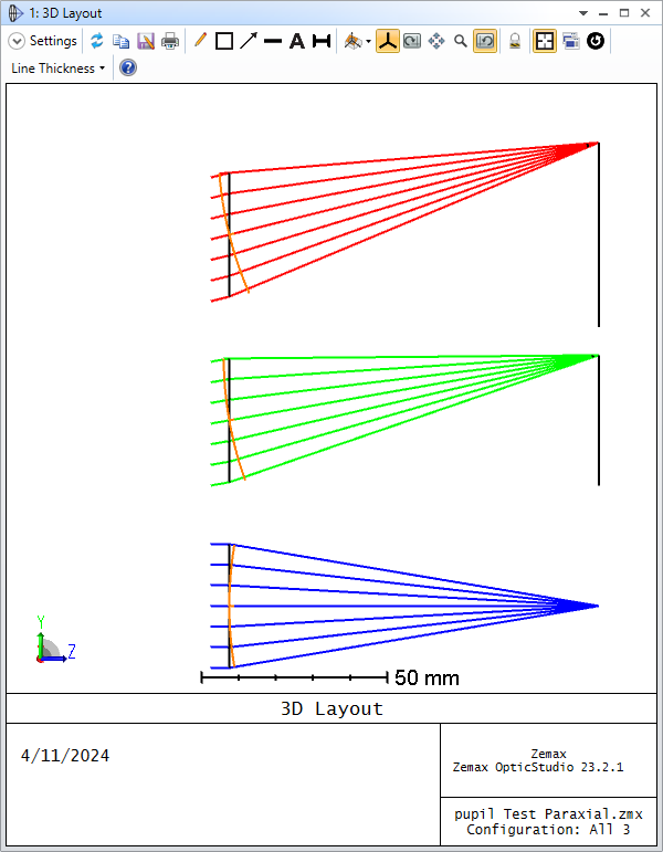
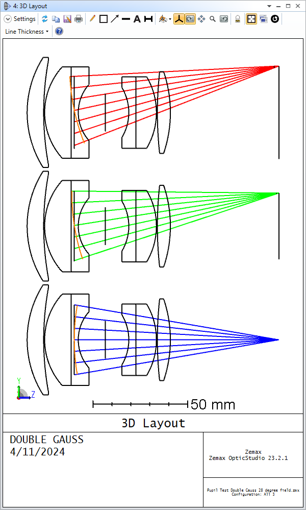
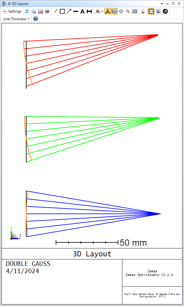
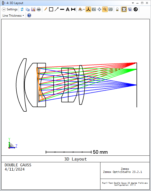
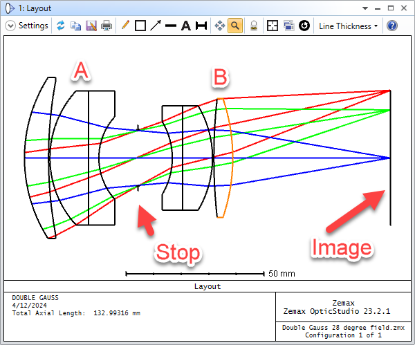
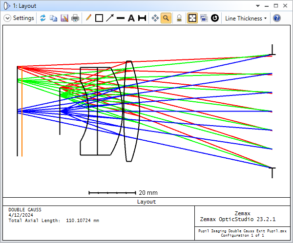
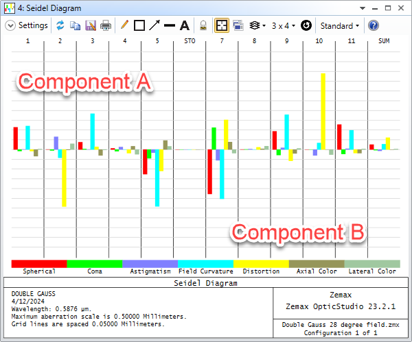
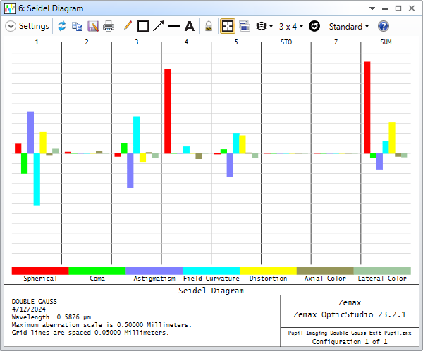
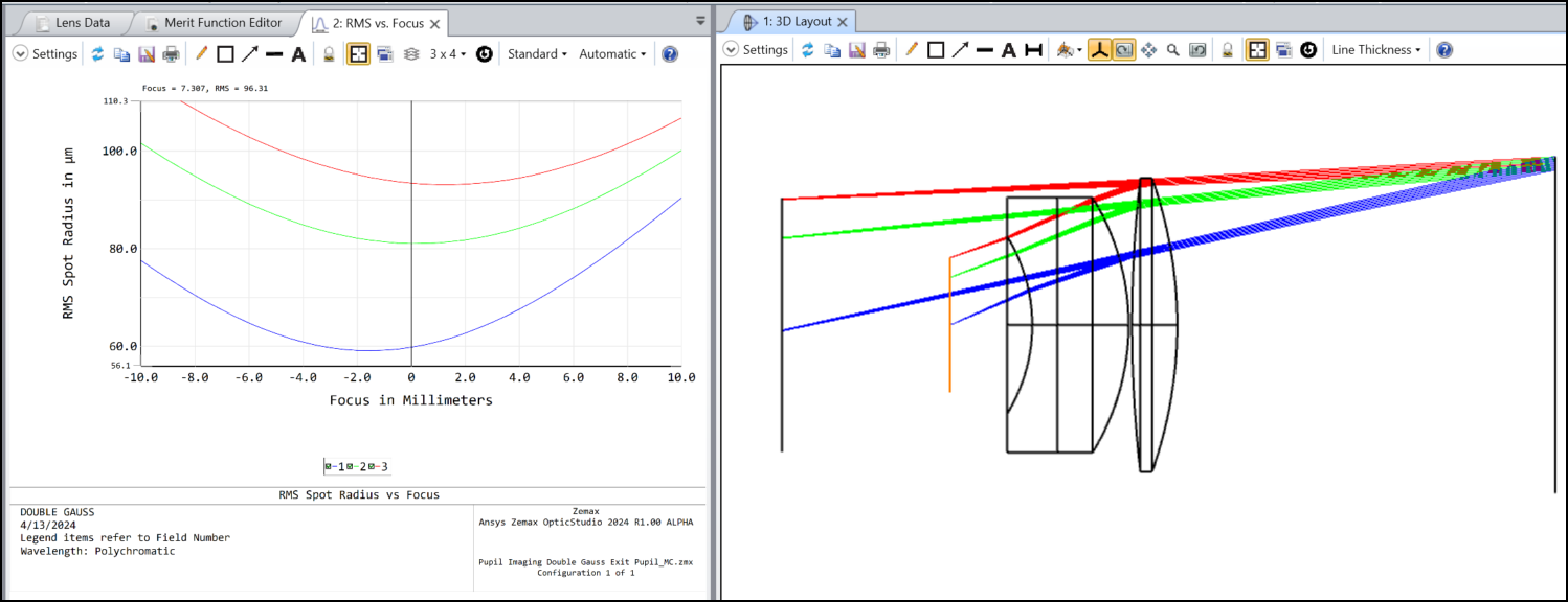
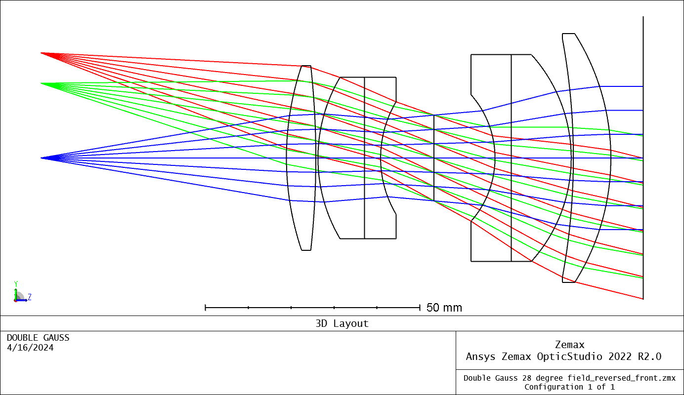
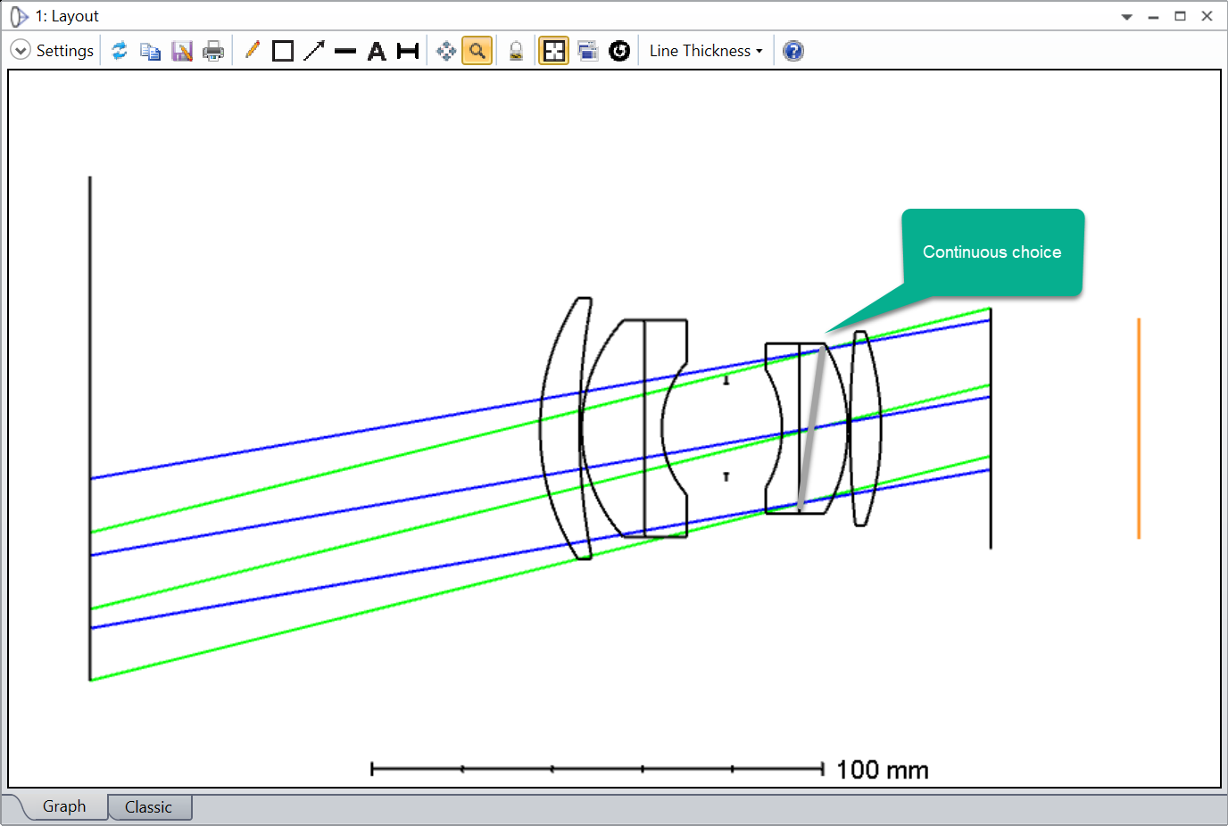
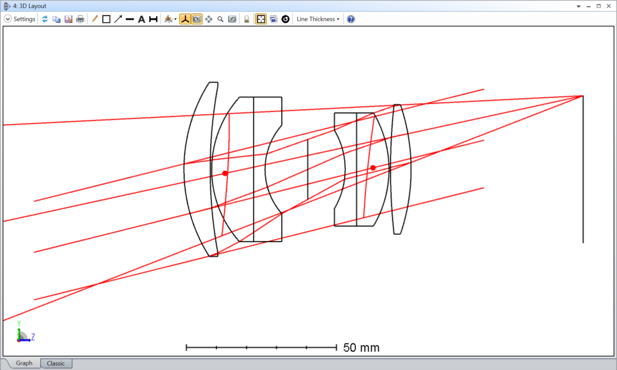
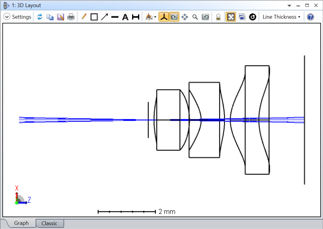
I can’t play with the feature to satisfy myself. Could someone post this layout (its the double Gauss sample file) with ‘Draw Marginal and Chief Rays’ selected please?

  • Mark

26 replies

Userlevel 7
Badge +3

BTW, in the KB article on the subject, it says:

Ray Aiming must be used to use this tool. If Ray Aiming is "Off", an error message "Field dependent pupil calculation requires Ray Aiming" will be displayed on the 3D Layout and the layout will not be displayed. The Figure 8 shows a 3D Layout when the Ray Aiming in the sample file "Double Gauss 28 degree field.zmx" is set to "Real" and "Draw Real Entrance Pupil" is set to 32.

Can I repeat my request that Ray Aiming be defaulted on? It was only ever defaulted off because back in the days of 286 and 386 processors it was an overhead that was not always needed. Nowadays that is not an issue and there’s no reason to not have it on.

Userlevel 7
Badge +3

OK, so using good old steam 23.2.1 I built the attached file. It’s the double Gauss, but with a dummy surface after the image is formed that tracks back to the pupil and draws it, then goes back to the image surface. I have to use multi-configs to have a configuration per field, but here is config 3, 14 degree field (hence 28 degree full field)

Now I’m just calculating this with chief rays so I expect your calculation to be more accurate than mine, but this shows the off-axis pupil

  1. Centered on the ray bundle of off-axis rays
  2. ‘Pointing towards’ the image surface as rays have to leave the pupil and form a point on the image surface. The one from the LinkedIn post is curved in the wrong direction.
  • Mark
Userlevel 7
Badge +3

One last post and I’m done :-)

This is showing all configs, and rays colored by configs. The blue rays are on-axis, red at the edge and green is the intermediate field. You can see the pupil decenter and tilt as a function of field.

If I recall correctly, Michael Cheng wrote a macro that computed pupil positions, tilts and sizes as a function of field. What does that macro show for this file?

  • Mark
Userlevel 6
Badge +2

Hi Mark,

Thank you for comment. Please find the following picture, which I think is what you are looking for. As you can see the marginal ray passes the entrance and exit pupils.

Feel free to let me know if you have any more questions.

Michael

Userlevel 7
Badge +3

Thanks @Michael Cheng . The curvature of the exit pupil is surely pointing in the wrong direction, no?

Userlevel 6
Badge +2

Hi Mark,

Thank you for feedback!

The results are found by searching for the focus. The following picture shows the concept. Note I use a larger perturbation at the field space for visibility. In the calculation, we use the much smaller one so the exact position would be different to what you see in the following picture.

I think the result basically shows the aberration (field curvature) at this subsystem. The circle drawn in your demo is used for calculation of wavefront, but it’s probably not the place with least aberration.


Userlevel 4
Badge

Hi,

Below image shows exit pupils for US07196855-1.zmx (attached as .txt, the forum does not allow .zmx attachments). It’s one of the many files from lens-designs database (https://www.lens-designs.com/photographic-primes)

That exit pupil for the red field looks very distorted.


Userlevel 6
Badge +2

Hi Ray,

Yes, this is exactly what we explained in the article: Paraxial vs. Real pupils in optical system – Knowledgebase (zemax.com) in section Distortion in real pupil.

I use some trick to draw the following picture where I send rays from a point on top side of stop and go to a ring sampling on the off-axis field you showed.

Now if I check the XZ view, you can see this pupil point actually has strong astigmatism. This is actually true for many other systems where the STOP generally don’t have a good focus and different definition give you different result.

In below, you can see the result for center and lower point.


And when try to find a focus, we must have a definition. Ae explained in the article, we use the “nearest point” to these rays as the answer.


I’m thinking to make the result more matching to what people would expect, we might need to have options to say they only want to find focus in tangential or sagittal direction. This will work for cases where we have strong astigmatism. But if the rays just don’t focus (telecentric), note we still just cannot really define a meaningful pupil.

That would be good to get some more feedback and thought from you guys. Although we cannot promise whether it will be added, I’m interested to see if you have any different comments.

Thank you very much for your input!

Userlevel 6
Badge +2

Hey Michael,

Thanks for this explanation.  If I can summarize, this feature is more analogous to the Pupil Aberration Plot, but rather than plotting aberrations in the XY plane, this feature plots it in either the XZ or YZ plane.  Is this correct?

Because this brings up my second thought...why is this important?  It’s not used in diffraction calculations (it’s on in the Layout Plots).  Your article mentions that EXPP uses paraxial rays but I’m 99% sure that OpticStudio uses real rays for the Exit pupil location (the Entrance pupil does use paraxial rays because sequential mode cannot perform a “reverse” ray trace).  I believe the EXPD operand also uses real rays, but only in the +y direction so the “ideal” Exit Pupil can be circular. 

If memory serves me correctly, OpticStudio currently uses this exact real ray approach to find the Exit Pupil location (it only traces parabasal rays around the Chief ray to find the location and your approach extends this concept to all pupil rays), but then when we look at diffraction theory, we need to consider the OPD between the perfect reference sphere which will give us the Bessel function (PSF) and the aberrated wavefront.  So would a distorted Exit Pupil simply change the circular boundary applied to the wavefront in the Exit Pupil?

So besides “why”, my technical questions are:

  • Why does EXPP and your code provide different locations of the Exit Pupil?  Having 2 different codes ostensibly calculating the same value is very concerning.
  • Why are you using normalized field coordinates to trace your 8 T/S rays?  I could imagine this becomes degenerate when you switch between field types.  For example, if I make the Double Gauss object distance 500mm, I can define the max field as either 14° or -139.407746mm.  If I now take the +0.001 normalized tangential field, it becomes 14.0014° or -139.4216867mm.  These are not the same 2 rays (14.0014° is equivalent to -139.422258mm and -139.4216867mm is equivalent to 14.001345°).  These will very quickly diverge if the working distance is large or the field is very far off-axis.

I could see this being really useful for wide angle systems to help with Ray Aiming, but unfortunately you need Ray Aiming for this to work in the first place.  

Userlevel 4
Badge

Hi Michael (H),


For the “why”, I can give you an example of why I used it today with this 3-lens system: I have been doing  raytracing to create images of a complex system seen through a typical miniature camera. This can be done in LightTools using backwards or hybrid raytracing (sending rays from the sensor towards the scene to meet either the light sources or the rays coming from the light sources onto the scene). To speed up the process, I may only launch rays through the exit pupil of the camera as to not trace rays that would “exit” the camera. Using this new feature, I could check if the paraxial exit pupil is a good aim area to use for all fields. For this lens above, it is, but I have another 2-lens system for which the paraxial exit pupil is way too small for the off-axis rays.

Userlevel 6
Badge +2

How would you then use the information?  You would simply use the H/V mouse coordinates as you however over the Layout Plot?  I guess my “why” is more of how is this implementation (decoupled from the MFE or an analysis that can be run via the ZOS-API).

For backwards ray tracing (assuming refractive/reflective system without diffraction gratings or GRIN), I simply flip the entire lens around and now the detector is your object plane.  Then knowing your NA in image space, you can launch rays from different image points and see the angular distribution.  You can then use this for your LT simulation.  

It would be incredibly helpful if OpticStudio had a full featured Reverse Entire System tool.  Currently, if you have any fields defined as Real Image Height or Paraxial Image Height, OpticStudio has to perform an optimization to determine the starting LM (and XY for finite conjugate) and this can be extremely slow (plus not even converge).  Also would help tremendously with Ray Aiming.

Userlevel 7
Badge +3

It would be incredibly helpful if OpticStudio had a full featured Reverse Entire System tool.  Currently, if you have any fields defined as Real Image Height or Paraxial Image Height, OpticStudio has to perform an optimization to determine the starting LM (and XY for finite conjugate) and this can be extremely slow (plus not even converge).  Also would help tremendously with Ray Aiming.

^^^^
This!

Userlevel 7
Badge +3

Hi everyone,

Well this has been a very interesting discussion and it has made me think a lot about the issues underlying it.Very good discussion, my thanks to all

Ray, I think your point is perfectly valid. I do expect systems like that to have highly distorted exit pupils, and its probably in the region where it’s not really helpful to discuss single pupils. But I think my concern is a great deal simpler.

I don’t have this feature in my version, and all I’ve seen in a screenshot of it being used with the double Gauss sample file. That screenshot has my spidey senses tingling though, as the pupil aberration just seems too big, and going in the wrong direction. Let me explain my reasoning again. Also, lets confine ourselves to the exit pupil, as it’s the easiest to access with an OS version that doesn’t support the new feature.


From the Help File, The Setup Tab > System Group (the Setup Tab) > System Explorer > Advanced Options (System Explorer) > Reference OPD > Exit Pupil

==================

Exit Pupil

OpticStudio by default uses the exit pupil as a reference for OPD computations. Therefore, when the OPD is computed for a given ray, the ray is traced through the optical system, all the way to the image surface, and then is traced backward to the “reference sphere” which lies in the exit pupil.

The figure below shows a singlet. The orange surface represents the reference sphere at the exit pupil.


The OPD at the Exit Pupil for a ray (Wave,Hx,Hy,Px,Py) can be simply written as:

OPDExit Pupil = OPDAbsolute + OPDCorrection

OPDAbsolute = OPTH(Surf=Object->Image Plane, Wave,Hx,Hy,0,0) - OPTH(Surf=Object ->Image Plane, Wave,Hx,Hy,Px,Py)

OPDCorrection = OPTH(Surf=Image Plane->Reference Sphere, Wave,Hx,Hy,0,0) - OPTH(Surf=Image Plane->Reference Sphere, Wave,Hx,Hy,Px,Py)

where OPTH is the Optical Path Length.


The OPD as measured back on this surface is the physically significant phase error important to diffraction computations, such as MTF, PSF, and encircled energy. This is shown in blue in the image below.

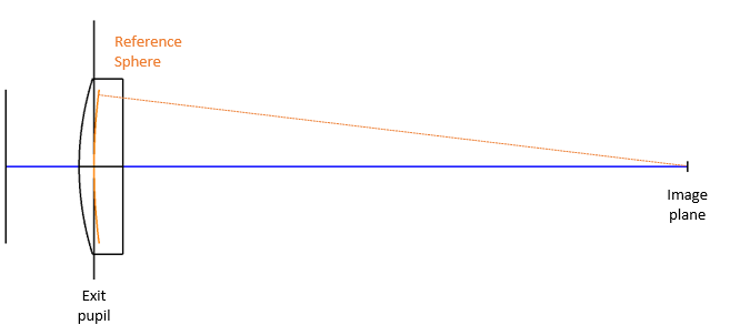
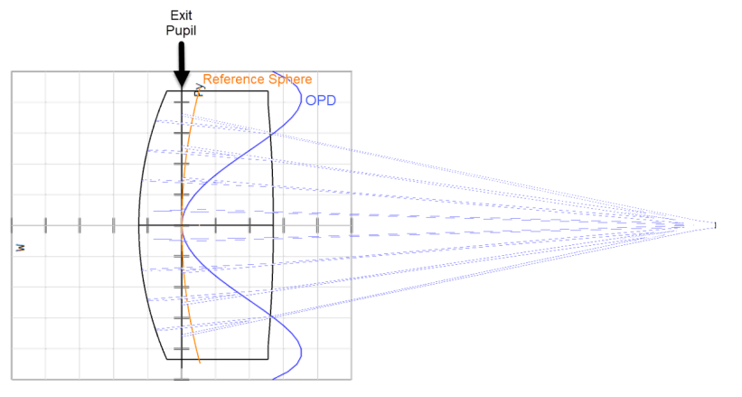
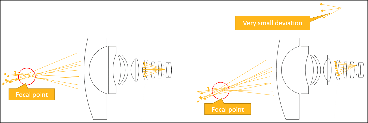
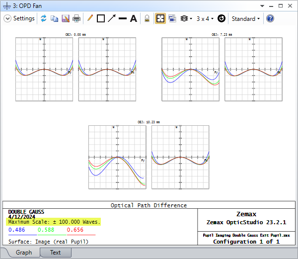
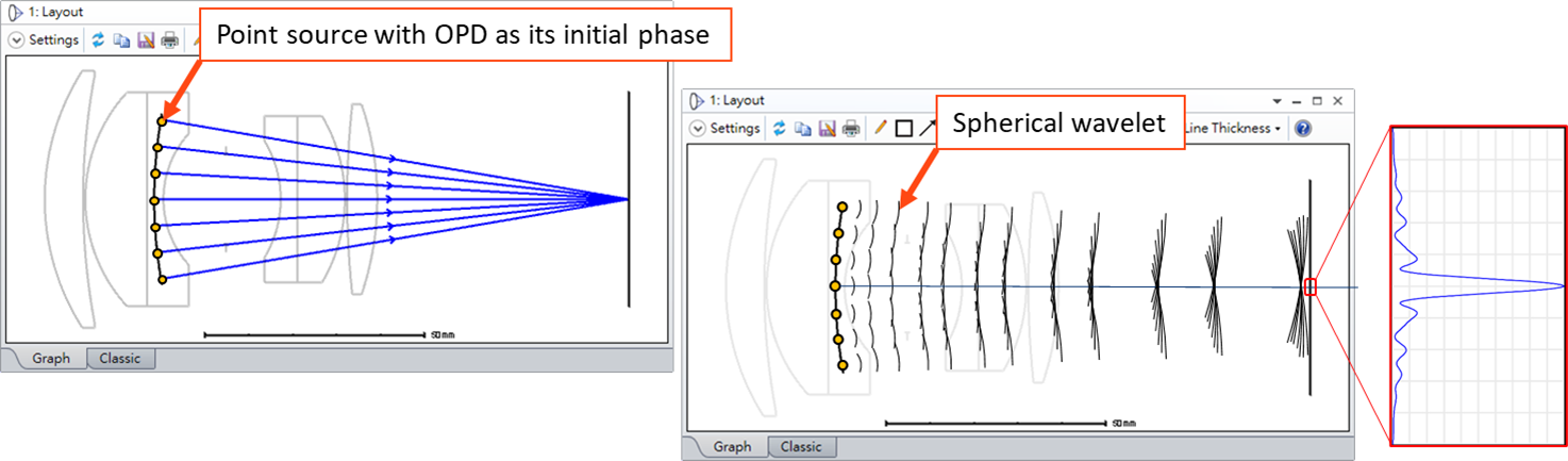
The additional path length due to the tracing of the ray backwards to the exit pupil, subtracted from the radius of the reference sphere, yields a slight adjustment of the OPD called the “correction term”. This computation is correct and is the desired method for all cases of practical interest.

=================

Note the distinction drawn between ‘pupil’ and ‘reference sphere’. I did not make that distinction earlier. I’m going to assume that everyone is happy with that definition. Please say if you’re not, as this is a foundational assumption.

Then, look at the paraxial test case in the zip file. This is just a paraxial lens with the same f/# and EFFL as the double Gauss sample file.

Since there’s no optics between the paraxial lens and the image surface, the exit pupil and lens aperture are the same, and what we’re seeing is the chief-ray centered reference sphere tilting in the untilted pupil. 

Can you (Michael C) confirm that the new code agrees with this? If it doesn’t, I think we have a real problem, but I’m going to assume it does, and move back to the double Gauss.

The double Gauss is a well corrected, moderate angle system with a few percent entrance pupil aberration shown on the Pupil Aberration plot. Because of symmetry, I expect the exit pupil aberration to be similarly small, but maybe I’m wrong to do so. Field Curvature is ~0.3 mm, the Petzval radius is ~-623 and distortion is less than 1%.


Here’s where I make the exit pupil location and reference sphere to be as a function of field, just using chief-ray follow solves:

I’ve used the magic of the Draw tab to hide all rays except those from the exit pupil, the reference sphere and the image surfaces. That’s why at the edge of the field the rays appear to miss the lenses. Showing just from the exit pupil gives:

Now I do expect the new feature to show a different, improved and more accurate calculation of the pupil locations than my simple chief-ray follow solves show. But I expect, maybe wrongly, differences of a percent or so. What I saw in the screenshot posted on LinkedIn was:

This shows the pupils moving by about 10 mm. I honestly did not expect to be able to see pupil shifts on a layout at all. How are we getting shifts of 10 mm on a lens with EFL 100 mm and moderate aberrations? Here’s my version of the results laid out the same way:

I just don’t understand why the pupil shifts are so large in this lens. And I’m sorry for being a pain...I have a well-documented history of keeping stubbornly at it until I understand something!

  • Mark
Userlevel 7
Badge +3

Ooops...I forgot to attach the files. Now attached.

One last piece of data. Look at the Power Field Map:

The EFL varies from 99.5 mm on-axis, which is the paraxial value, to 99.2 at the edge of the field. That’s .3 mm variation in focal length. How then do the pupils shift by 10mm?

  • Mark
Userlevel 6
Badge +2

Hey Mark, 

The only addition I would make is the Chief Ray Height uses the paraxial chief ray whereas the Pupil Position uses real, parabasal rays about the chief ray.  So I would replace the C with a U which would change the Exit Pupil position from -108.059574 to -108.06062.  

But I have the same fundamental question.  If using the Pupil Position solve gives -108.06062 on-axis, is there really a 10mm shift for a 14deg field?  Ignoring the aberrated pupil shape/curvature (so only looking at the chief ray) why is there 2 different code paths which are supposed to calculate the same value (Exit Pupil location) that are giving such different results.

Userlevel 6
Badge +2

Another “spidey sense” (I like that phrase Mark) is we know the Double Gauss is a pretty well corrected system.  Looking at the curvature of the aberrated Exit Pupil would imply the bottom marginal (green) ray travels a lot farther than the top marginal (orange) ray; I’m not sure this is supported with diffraction theory.  If this is really the pupil the individual rays see, then there would be significant aberration & tilt in the 14deg field.  This just doesn’t “feel” correct.


Userlevel 6
Badge +2

Hi Mark and Michael,

Thank you for nice discussions and good questions.

To answer them, I think the key point is to explain how it’s calculated and then we can compare it to the other method.

The calculation behind this feature is to find the focal point assuming we have a point source on the STOP surface, as shown in the following picture. For a specified point on the STOP (px,py), we choose 8 rays surrounding the center ray that points to the specified field (hx,hy) and find the focal point in 3D space.

On tip I think can be useful is maybe to ignore the concept of pupil and reconsider this is an imaging system where the original STOP is new object, although here we don’t really have an “image plane” but want to find the best focus in 3D space.


The rays we choose are the 9 as shown below.

Note the definition of the focal point is then important because in most of cases, these rays don’t perfectly converge to one point and different definition can give different result. In this feature, we take the point that has the smallest RMS perpendicular distance to each of the ray.


In the following discussion, I would like to assume we agree there is no bug and we calculate exactly as mentioned above; the drawing you see is the result of strictly following to the above rule. We then can focus on whether this is a good method and compare to other methods in the discussion.


Reason to perturb rays in field coordinate

Initially the plan is to use the angle deviation in object space then the result can be independent to the field type. However, we faced speed issue and scheduling pressure. It’s correct this means the result can be affected by both field type and maximum field. It’s a tradeoff of speed and accuracy.


Exit Pupil

It’s correct EXPP and EXPD are based on real rays. Sorry for confusion as I think it may be too much explanation to touch to this point. In most of cases, I think it’s no critically wrong to say it’s supposed to give you the “paraxial” data.

About the different of this compared to real pupil calculation here. I think it’s mainly about the selection of rays. Exit pupil only use y perturbation while the real pupil here uses 9 rays for every direction with the “nearest point” method to find the focus. The benefit of using more rays is we can catch more cases such like an off-axis and/or non-rotationally symmetric systems.

There are some other minor differences. For example, exit pupil does not use only a constant deviation, such like 0.0001 used in this real pupil drawing. Please allow me to skip to the details here, but I think this probably also contribute a little to this difference.


Pupil Aberration

Although I can see there may be some relationship, but I would say this is a different analysis than the real pupil drawing. This feature traces a ray from specified field and compare the ray position on Entrance Pupil and on STOP. The comparison is based on the “xy coordinate” on two plane. However, the difference you think significant is in 3D space.

This is just my explanation but hopefully make sense to you: If we consider an imaging system where original STOP is the new object and original entrance pupil is the defined new image plane, Pupil Aberration is then the distortion analysis and the real pupil calculation shows the field curvature. Note in this imaginary new system concept, the distortion is calculated by chief ray (single field in original system), while the real pupil calculation is calculated by something like centroid (RMS of distance to each of the ray).

I’m a little not sure if there is a clear math or concept to say, but I think it’s possible the system has only a few percent of chief ray based distortion but have stronger centroid-based field curvature.


Diffraction theory, OPD, PSF

This is a good question. The feature is not developed with targeting to improve anything in this point. I’m not sure if we can further utilize the result for it. I don’t know either if we should find any physical meaning with the difference between the “Reference sphere” we used for OPD and the real pupil we calculated here. From the result, we only know if you try to trace rays from a point on the STOP and find the focus in the image space, the best focus do is far from “reference sphere”. I think maybe it’s possible. We don’t have a theory to promise that, if a system is well-perform in normal object-image configuration, if must also have a good image quality between STOP, entrance/exit pupils, right?


Double Gauss

It’s mostly explained in previous points. My thought is we should first clarify how this is calculated, which I have done above. The links to Pupil Aberration and Reference sphere is interesting, but unfortunately I don’t have quite complete answers. I would actually then be wondering how do you think we should calculate in order to get a sense-making result as you would expect, other than the method we used here. I’m interested to hear any different idea!


Ray Aiming

I think it’s a “Chicken and the egg” question. We need Ray Aiming so I can do “ray tracing” from STOP. And I understand we hope Ray Aiming can get this data before it’s triggered.

If we want to help Ray Aiming with the way you imagined, I think what we really need to have is the true reverse ray-tracing from STOP.


Use Case

Here is what I know.

I think there are more, but not all users can share what they are trying to do.

Userlevel 7
Badge +3

Hey Michael,

Thank you for that. It sounds like the method you are using is similar to the Power Pupil/Field maps, in that you trace a chief ray at some field point and a ring of rays around it, and then find where the rays cross or have closest approach. The difference is you’re firing rays that start on the stop surface, then through the previous/subsequent surfaces, to find pupil locations.

I think that method is sound, but I just don’t like the answers it’s giving. It seems to me that there’s some bug lurking around somewhere. The shifts you’re seeing are just so large compared to everything else. This is my spidey sense, but I do have a track record on this 😀

I’d suggest building some simple test cases and experimenting further. I don’t have access to the feature, so can’t help more. I guess I have to just say that while the method sounds fine, I don’t believe the results you’re getting, and just leave it at that.

  • Mark


Userlevel 7
Badge +3

Hey again, Michael

Well, I just couldn’t leave it at that 😁, sorry. I’ve done a bit more thinking and I think I have found a flaw in the logic, or at least a candidate solution for you peeps to think about. 

Let’s start with the original Double-Gauss, which is made up of component A, the stop surface, component B and the Image surface:

I then

  • fixed all surface apertures,
  • deleted component A,
  • made the old Stop surface the new Object,
  • set Object Height as the field definition such that the object is the same size as the original d-G’s stop
  • Made the image surface the stop, it’s aperture unchanged,
  • Used Float-by-Stop, paraxial ray-aiming on,
  • Added a new surface after this new stop, and used a marginal ray height solve to place it. That should place this ‘image’ surface at the same location as the paraxial exit pupil of the original d-G
  • Added a new surface after that, and used Optimize...Quick Focus to locate it at best RMS wavefront error. I called that the ‘real’ pupil

This gave me the following:

Now the good news. You can see the paraxial image is located at -108.060 mm from the stop, and this is consistent with the original d-G’s exit pupil location of -108.064. I’ll take that. The ‘real’ pupil is shifted 2 mm away, and that’s consistent with the shifts the new algorithm is producing.

The bad news is that the lens is totally aberrated:

and this is where I think the problem lies. In the original d-G, look at the Seidel plot:

The overall system aberration is low because Components A and B balance each other out, leaving a small residual. But neither A or B is diffraction limited by itself. Here’s B as a standalone system

The aberrations of system B by itself are just not the same as the aberrations of the B-component of the full system. I think this brings the whole method of treating the stop surface as the source of rays into question.

It’s only partially true that the exit pupil of the whole lens is ‘the image of the stop’ seen through the final components. It’s actually the image of the stop as illuminated by the first components. You cannot ignore Component A! Another way of saying it is that the illumination of the stop is aberrated by component A, and this is accounted for when we optimize A and B together.

So, I don’t think this ‘rays originating from the stop’ method is the correct way to compute the pupil locations of a diffraction limited (or maybe any) system. I just don’t think this method is computing what we hoped it was computing.

  • Mark
Userlevel 6
Badge +2

Hey Mark,

Once again your instincts and insights are invaluable.  I think we need to slightly modify your file. 

First, we shouldn’t keep the image plane the same size; this would mean we’re tracing a full pupil but we know we should be tracing parabasal rays.  I decreased from 24mm to 4mm (we would go smaller but I want to visualize the ray trace).  

Then, I make the y-fields symmetric so I can actually look at the full pupil fan.

Next, I add a CB before the Stop to shift in Decenter Y...this allows me to simulate the different fields with the MCE.

Then, I add a second CB after the Stop to rotate with Tilt About X (make these variable)...this allows me to optimize the best plane representing the “real pupil”.

Finally, I set the Field Weight for all but the +/-10.229 fields to 0 and optimize.  This gives me the “best focus” “real pupil”.

Now that we can visualize (both mentally and in OpticStudio) what the “real pupils” are, this brings up a few more points:

  • We’re still talking about localized parabasal image points around a centroid ray.  The EXPP uses real rays and I think calling EXPP “paraxial” and the pupil visualization tool “real" is a HUGE disservice to the diffraction capabilities that Ken built into Zemax over 30 years.  The current Exit Pupil calculations are 100% correct, are not paraxial and I hope that Zemax marketing in the future really looks into their use of “paraxial” vs “real”, because one implies an approximation and one implies the ground truth.
  • As you pointed out, this is highly dependent on aberrations.  By only looking at the closest ray-intercept for back-propagating rays, this can easily lead to unstable solutions (especially for XP far away from the image plane where the ray intersection runs into numerical rounding issues)
  • This feature makes the “Stop” seem like it’s an object or image plane but in reality, it’s the physically limiting size of the converging wavefront in image space.  This “physically limiting size” is what causes the PSF (vs a perfect point source) and since it can’t be defined by geometrical rays (that’s why OpticStudio has POP...see Zemax\Samples\Physical Optics\Gibbs Phenomenon.zmx), I think using rays in this manner is misleading.

One last thing to note is that by boiling this down to the 2 extreme marginal rays, we can see this becomes a Scheimpflug object/image tilted scenario.  But as I pointed out, the Stop itself isn’t a plane, but rather a limiting aperture.  So rather than having a tilted “real pupil”, we could tilt the Stop (in orange) to the “real pupil" is flat:
 

However, for the actual rays in the system, they don’t see a tilted Stop, the rays simply see an elliptical Compressed and Decentered aperture (analogous to Vignetting Factors).  

So while I can see use of this feature in particular cases, I’m worried the marketing and documentation around this is lacking.  The impression I got when I first read the Release Notes is this is showing the “correct” Exit Pupil when in reality it’s showing the “geometric aberrated aperture”.  I think replacing the terms “real” with “aberrated” would go a long way to not implying the actual diffraction calculations are incorrect.  

Userlevel 6
Badge +2

Hi,

Thank you very much for feedbacks. As Michael H explain. I have also built a similar file with the RMS vs. focus where also shows the focus shift from upper side to lower side.

For the naming of paraxial and real, I think it’s a good question and thank you for pointing this out. I understand many of these quantities are actually calculated by real raytracing. Almost all quantities that users use as paraxial approximation, as described in book, in Zemax OpticStudio is in fact not strictly calculated under paraxial approximation but by tracing very small angle rays, which although is also “paraxial”, numerically. We can change all the documentation to emphasize this everywhere, but I can imagine that will probably confuse other users who are not aware of the differences. We will probably need to clarify more anyway.


Thank you for providing the name of aberrated pupils. I like this name. Unfortunately, I didn’t learn this one earlier otherwise I guess we can have a vote internally. :) 


On the other hand, I would like also mention that the current method can also handle for off-axis and non-rotationally symmetry system as the calculation is not only for y direction. Hopefully this can be a good information for some use cases.


I learnt from this discussion this feature may not be as you expected for some other cases. But I wonder if you have other way to calculate. It seems to me at least we agree it should be rays from a “single point” on the STOP right? My understanding to the idea of “illuminated by component A” is that means different ray sampling, but not sure if there is a good way to apply this concept. Or from the first discussion, it seems to maybe what some people would expect is actually a feature to draw “Reference Sphere (OPD)”?

Userlevel 7
Badge +3

Hey Michael(s),

Thank for this discussion. I’ve taken a few days to reply as I wanted to think deeply about this.

I think what is needed is a lot simpler than what has been implemented. We want a plot of the entrance pupil as a function of field, because in wide angle lenses the pupil shifts and this is what makes ‘wide angle’ lenses work. In a sense, this is not aberration in that the pupil shift is a desired effect, in much the same way as lateral color is not an aberration in a spectrometer.

Doesn’t the location of the real entrance pupil just drop out of the ray-aiming algorithm? What is the ray-aiming algorithm aiming at, if not the non-paraxial pupil? I think this is the desired information.

For the exit pupil, it’s easy enough to compute real pupils using pupil solves and chief-ray-follow solves. But again, it is the plane in which the reference sphere is placed, so again I expected this to just drop out of the work OpticStudio already does with the field-dependent exit pupil. Since we’re after the stop we know which rays are the chief and marginal ones and the result isn’t so difficult.

The new algorithm, that treats the stop as a source of rays is flawed for the exit pupil as it ignores the aberrations of the entrance pupil and of the surfaces prior to the stop.

I think the questions that should be answered are:

  1. If you were on some patch of object surface, where should rays be aimed to get through the system if the paraxial exit pupil is not a good enough first guess. This is exactly what ray-aiming does, we just need access to the data it already has
  2. For the exit pupil, where is the plane that houses the reference sphere as a function of field?
  • Mark


Userlevel 6
Badge +2

Hey Mark,

I remember one of the computational physicists saying that if they could rewrite any part(s) of the source code from the ground up, would be sequential ray aiming and non-sequential gradient index ray tracing.  So I don’t think Ray Aiming actually “calculates” the real entrance pupil, rather it simply uses a shift from the paraxial entrance pupil to find any ray that makes it to the Stop.  Once it finds this ray, it doesn’t ray to back calculate the real entrance pupil.  The EP is used for setting up a ray while the XP is used for diffraction calculations, so in terms of calculations, the XP is significantly more important to get “correct”.

Rather, for Ray Aiming, I think this is where the Reverse System would come into play. 

You would reverse the front half of the system, make the Stop the modified object plane, place a Coordinate Break and dummy surface directly before the new Image Plane & make the dummy surface the Stop.  Now with Ray Aiming on, simply move the Stop in Decenter X & Decenter Y.  With sparse sampling, you can build up a map of acceptable input angles which actually make it to the stop while only performing forward ray tracing.

From this you can see that a ray angle of 33.62deg fails to trace but 32.17deg is traceable:

Going back to the original Double Gauss and plugging in the numbers, you can see the lime ray traces while the blue doesn’t:

This technique would replace the “grid search” part of the Ray Aiming algorithm since there would already be an Angle+ObjectHeight mapping of acceptable values.

This would fail for UDS and care would need to be taken for Birefringent & Gradient Index materials, but for refractive/reflective systems this would have a 100% success.  

Now for the second question, I don’t believe the z-position of the exit pupil plane changes.  The field dependence for OPD calculations comes from a) the oblique “correction term” and b) the chief ray-to-image plane distance (radius of the reference sphere).  As Michael C pointed out, I remember the Exit Pupil is only calculated with a +y field value on-axis.  This affects wavefront & FFT calculations, but since these analyses are looking at the difference of optical path lengths and the phase will have a 2pi modulus, I’m not sure how big the impact is.  The good news is I don’t believe the Huygens integral uses the wavefront directly, it simply uses the cumulative OPL on the image plane, so our “golden standard” diffraction calculation is unaffected by the XP location.

@Michael Cheng 

Can you confirm the following:

  1. In System Explorer > Advanced > Reference OPD, the Exit Pupil calculation always uses the on-axis Exit Pupil for Wavefront/FFT calculations?
  2. The Huygens algorithm does not use the Exit Pupil OPD reference, rather the Huygens algorithm uses Absolute/2 OPD reference?
Userlevel 6
Badge +2

Also, if I look at the “field dependent” Exit Pupil, I get slightly different planes.  For each field, I manually get the following offset:

  • 0deg : 0mm
  • 10deg : -2.5mm
  • 14deg: -5mm

Since the Double Gauss is only defined with +y fields and is rotationally symmetric, I can mirror these fields to the -y axis in order to get 2 exact chief rays for each field and then find their point of intersection (the “true reference sphere”).  This is a simple example and only works for rotationally symmetric systems, but I’m surprised to get such a big difference (about 5mm) for the 14deg field:

Overlaying this with the 24.1 Layout, you get the following differences where the orange planes going from right to left correspond to the blue, green, & red Exit Pupil locations:


Userlevel 6
Badge +2

Hi Mark and Michael,

Thank you for feedback and discussion. Sorry I might be slow as I’m a little overwhelmed recently.


I think it’s a good question about where the Ray-Aiming should target to. The following flow of thinking is the same concept as I explained before, but hopefully it gives you different viewpoint why it looks like this. 

If we look at only one field, this plane for Ray-Aiming to target can actually be arbitrary as long as it covers the edge. The following choices all work.


I think the another rule we implicitly apply is we want these real/aberrated entrance pupils are continuous between neighbor fields. So, we actually want to make a little perturbation in field and then look for the interceptions. This makes sure the choice continuous to the neighbor fields.  The following shows an example, where I perturb the field in y direction. Note this is only in y direction.


Now if I try to include more perturbations in 8 directions. (For only px=0, py=1) You can find we have quite different focus in YZ and XZ view. This means the strong astigmatism exists. I think it’s the reason of discrepancy seen in Michael’s comparison. In this case, what we do is to find a nearest point that satisfy all these rays.

I think this is an inevitable result if we choose to have a point source on the STOP surface. As Mark thinks, maybe we should somehow consider “the other half” to compensate this, but I don’t know if there is any physically meaningful consideration to this problem.

I was thinking maybe we should also provide an option for only using perturbation in tangential and only in sagittal. I think what Michael calculates is the focus in tangential direction. However, as mentioned before, we have schedule pressure and we cannot include too many ideas. :)

(I believe you all know, but I use trick of raylist.txt to draw this by the way, for reference of other readers.)

Just by the way, one user has shared to us that in his experience, this STOP aberration is a true problem. It happens when you want to measure the F/#. The image of STOP is blurred so they might need to discuss with their customers what is acceptable definition.

The other very unmature thought I’m thinking is maybe somehow we should first decide a plane and just draw the centroid of these perturbation rays on this plane. It seems to me users would more expect a plane-like pupil, not a so aberrated in 3D space. But I don’t have any physical viewpoint about how this plane should be chosen. This is probably just a bad idea.


I agree the reverse trick should be a good trick to speed this up. Maybe we can build a twin but reversed system in the background and always use it to assist Ray-Aiming. I also agree this will be limited in many ways. In addition to DLL, I also think it will be problematic to correctly reverse a system with CBs. We don’t really handle this case well so far.


For the following 2 questions:

In System Explorer > Advanced > Reference OPD, the Exit Pupil calculation always uses the on-axis Exit Pupil for Wavefront/FFT calculations?

This field dependent pupil is really only used in drawing for now. (There is a discussion whether we should have operand to give exact number.) So I think we do just use on-axis Exit Pupil as before. (as Mark explained in very initial replies.)

If needed, I can double check in core, but I may need a little time.
The Huygens algorithm does not use the Exit Pupil OPD reference, rather the Huygens algorithm uses Absolute/2 OPD reference?

I think this depends on which method is chosen. For Force Planar we use just the OPL as is when it reach to image plane.

For Force Spherical, I have a picture to explain the concept that we do use the reference sphere.


Reply