Question

Deriving Ray fan plot from OPD plots

  • 11 July 2023
  • 3 replies
  • 315 views

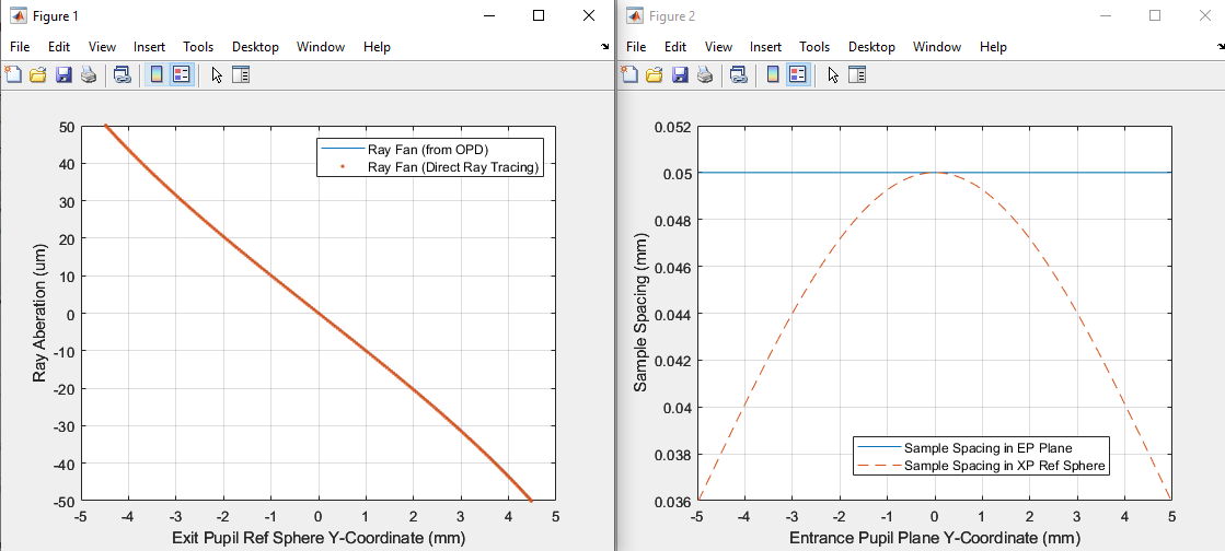
Can somebody help me to understand how to get the ray fan plot from the OPD plot?

In the case where i only have defocus and some piston as wave front errors, the first derivative of the OPD curve (polynomial of 2nd degree) should lead me to a linear function, describing the slope of the OPD at any pupil coordinate (independent of the piston, since it doesn`t change the slope of the OPD curve).


However, whenever i try to calculate the ray fan value at a certain pupil coordinate, it always deviates from the value thatis shown in the ray fan plot at that point. Why is that? Maybe i am making a thinking error.

My recipe would be as follows:

  • Read coordinates of  max. pupil coordinate point of max. field in OPD plot. (both in mm for example)
  • calculate coefficient “a” of function   OPD-value = a * pupil-coord. ^2    (since its a pure defocus)
  • Calculate derivative of quadratic OPD function  (which gives me the linear ray fan function)
  • Calculate value of derivative of OPD function at max. pupil coordinate
  • → should agree with value in ray fan plot at the same pupil coordinate

Thanks a lot for your help


3 replies

Userlevel 7
Badge +3

Hi Sandronium,

As you know, the ray-fan plot is the derivative of the OPD. We trace a ray to the image, and look at how far it lands away from the chief ray. The error in x and y are given by


error_x = -(R/n)(dW/dx)

error_y = -(R/n)(dW/dy)


where W is the wavefront error (OPD) R is the reference sphere, and n is the index of propagation.


So W is measured at the pupil, and error_x,y at the image plane.


I'm not sure where your calculation is going wrong, but at least we know that the OPD and ray fans as computed by OpticStudio are correct: yes?


My algorithm would be something like


create a dummy surface located at the exit pupil. Use a pupil position solve for this

trace a ray hx, hy, px, py, wavelength

then trace four more rays, at +/-delta_x, +/-delta_y around this ray. Make the deltas small.

compute the gradients of W at the exit pupil location in x and you from these five rays

scale by the distance from the exit pupil


You should then have ray landing coordinates on the image surface that agree with the ray you traced.


  • Mark
Userlevel 7
Badge +3

This is an interesting question.  I have a few more details to add to Mark’s previous comments.

First, out of curiosity, I looked at a couple of example lens models.  I began by simply copying the y-direction OPD data directly from the OpticStudio OPD Fan analysis window into Matlab.  I then converted the normalized entrance pupil coordinates to exit pupil plane spatial coordinates (via a simple linear scaling), and used these to calculate the numerical y-derivative of the OPD.  Upon applying the standard equation to find the corresponding ray aberration, I too found a disagreement with what OpticStudio reported in the Ray Fan analysis window.

After more careful consideration, I realized the problem.  It has to do with the pupil coordinates used to calculate the OPD derivative.  Let’s consider just one direction in the pupil, say the y-direction.  When calculating the OPD derivative, what exactly is the y-coordinate?  It’s actually the y-coordinate of the ray intercept on the exit pupil reference sphere, not simply a linearly scaled version of the entrance pupil coordinate applied to the exit pupil plane.  The entrance pupil sampling is typically uniform (unless a non-uniform aperture apodization is selected).  However, the exit pupil reference sphere sampling is non-uniform, with the non-uniformity increasing as the lens NA increases, so it can, in general, become quite significant. 

It therefore seems that the best way to get the OPD data along with the correct exit pupil coordinates is to use a ZPL macro.  As Mark noted, in your lens model you can propagate rays to the image plane (say with defocus if you like), then back propagate to the exit pupil reference sphere.  The pertinent ray data and OPD data can then be generated and output to a screen window.  At this point I find it easier to copy the OpticStudio data into Matlab for further processing and plotting.  The details, along with results for an example aspherical lens, are attached.

Here is another simple example using a paraxial lens with pure defocus:


After ZPL data collection and processing in Matlab, here is what I find:

The ray fan aberration data on the left is plotted against the Exit Pupil Ref Sphere Y-Coordinate, so the result is not a perfectly straight line (like it would be if plotted against the entrance pupil plane y-coordinate).  However, the agreement between the ray fan computed via the OPD data versus the direct ray trace fan data is quite good.  The non-uniformity of the Exit Pupil Ref Sphere y-coordinate sampling is shown on the right.  A closer look at the ray aberration plot shows a very slight difference between the computed and direct results, seen here when zooming in:

which can be attributed to the fact that the exit pupil reference sphere radius is used for “R” in the equation, when in fact the exact result requires use of a slightly different distance (see the detail in the attachment). 

So, getting the correct result requires understanding exactly what the (x,y) pupil coordinates are in the well-known equations relating the OPD derivatives to the ray aberrations.  This is an important detail that I didn’t fully appreciate until working through these examples.

Regards,

Jeff

Hi Jeff and Mark,

Thanks a lot for your detailed answers. I really appreciate your efforts. 

Your explanations helped me very much.

Best regards,

Sandro

Reply