Solved

Comparison of POP results and Paraxial Gaussian Beam Data

  • 11 February 2022
  • 9 replies
  • 800 views

Userlevel 2

Dear Experts,

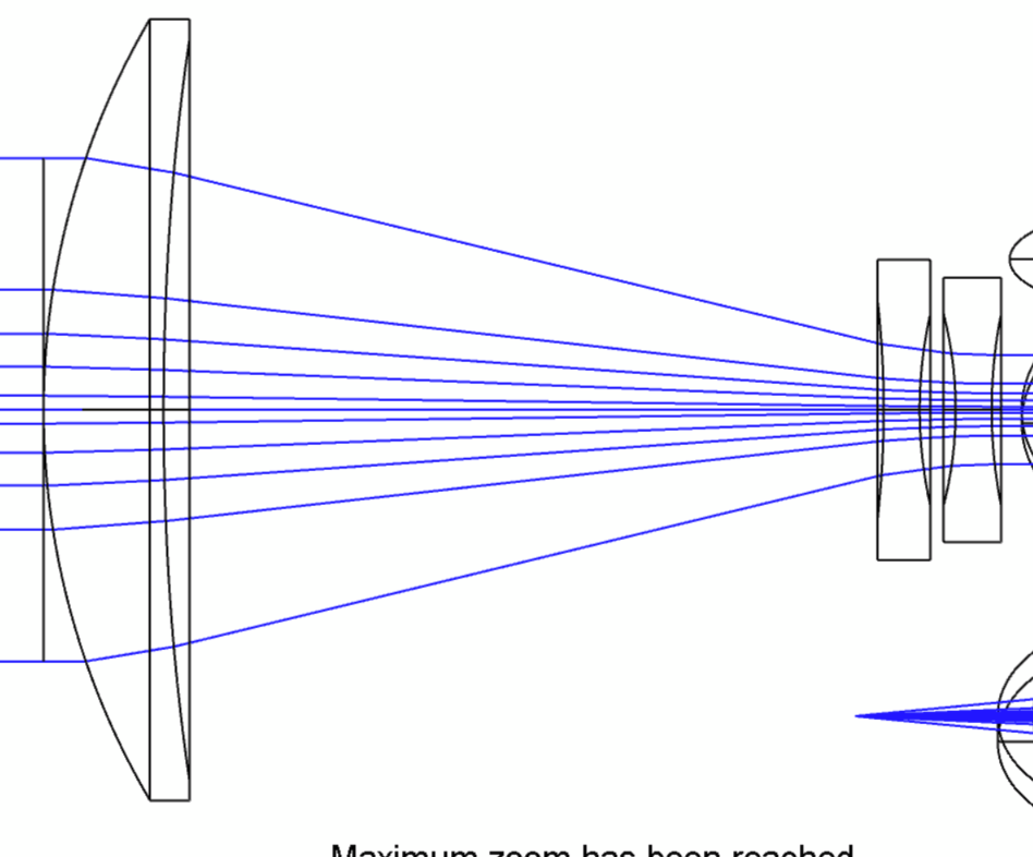
I have collimated a single-mode fiber (mode field radius 5.2um) output with a collimating lens and a beam expanding telescope. I propagate the beam over a long distance.

To check the collimation (and later do some tolerancing analysis) I have used a Paraxial Gaussian Beam Analysis:

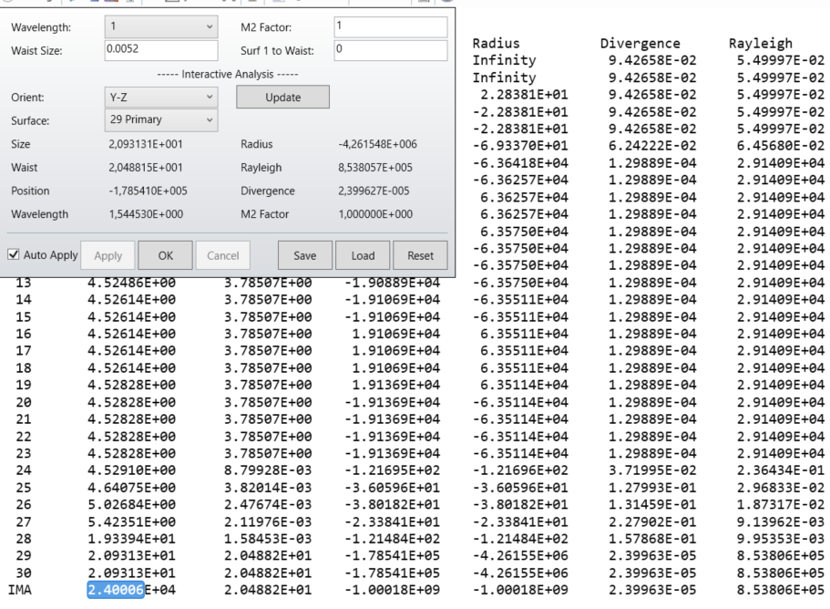
Surface 29 is the output of the telescope. I have a divergence of 23.99urad and a beam size (radius assuming 1/e²) of 20.931mm. Propagation distance is 1e9mm, which gives me the 24m (my paper calculation) in agreement with the IMA beam size (radius). So far as expected.

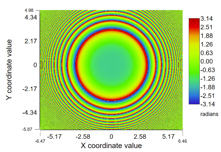
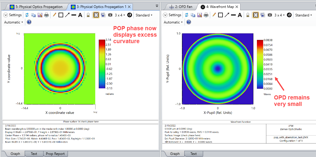
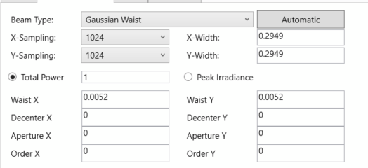
Now I do a POP propagation:

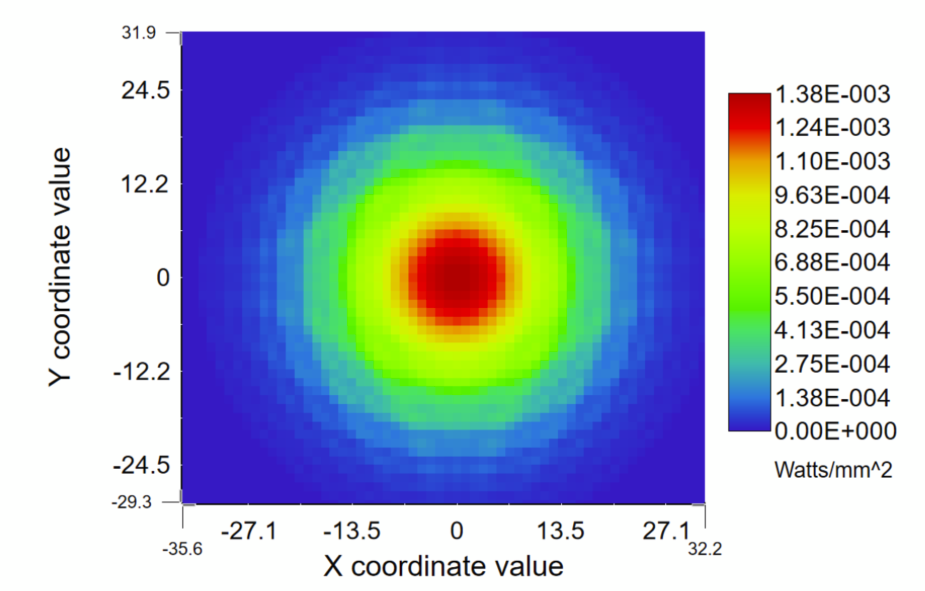
Beam irradiance at surface 29 looks a bit disturbed, but not too bad, and it confirms the 20.9mm beam radius:

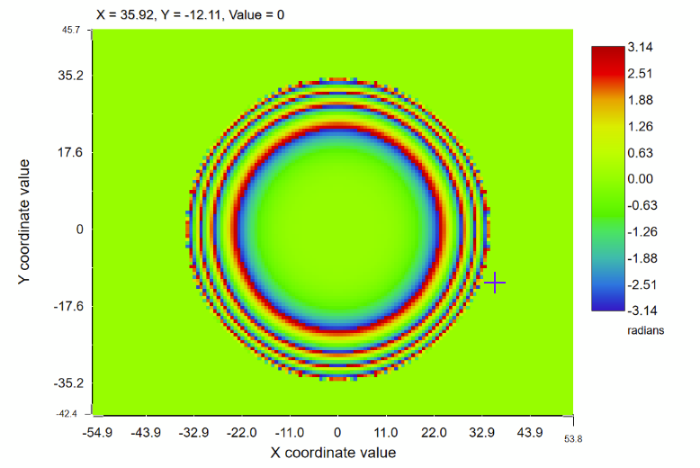
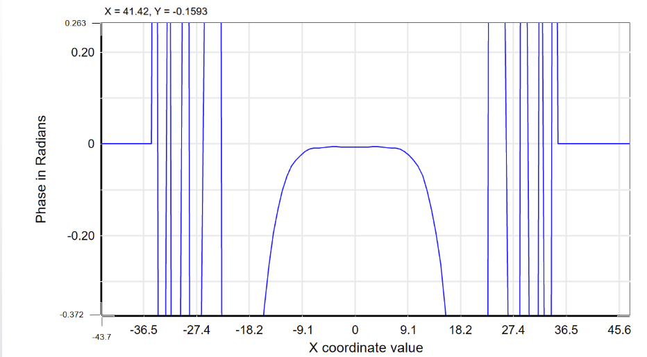
In the IMA plane Surface 31 I get the following graph:

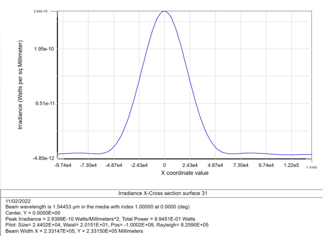
The pilot size (shown on the bottom) is 24.4m (close to the paraxial results and what I would have expected from the divergence). The beam width is shown to be 233m? Not sure what this means. If I look into the cross section graph and estimate the 1/e² point, I get something like 42m beam widths (radius) or 84m (diameter). So I see 3 different values for the beam width 24.4m, 233m, and 42m.


My system contains a couple of flat fold mirrors. I understand from the manual, that tilted flat mirrors are ok for the Paraxial Gaussian Beam Analysis, right? Otherwise the system contains lenses with spherical and even aspheric (4th order) surfaces.

Many thanks for some hints.

Markus


icon

Best answer by Jeff.Wilde 11 February 2022, 22:38

View original

9 replies

Userlevel 2

On the surfaces of my telescope I seem to get aliasing effects in the phase, which maybe makes my results invalid. I have already turned up the resolution to 4096x4096.


What could be the work-around for this? Is there any possibility to calculate the irradiation distribution in the far-field, if POP fails due to aliasing effects? Can I nevertheless trust the Paraxial Gaussina Beam analysis?

I would have liked to use this analysis in a Tolerance analysis with Monte-Carlo Overlay graphs to show probable irradiation distributions in the far-field.

Many thanks

Markus

Userlevel 7
Badge +3

Hi Markus,

1. For your first question about beam width, see the definition:


In your beam irradiance cross-section, it looks like you have a small, but non-zero background irradiance.  If that is indeed the case, and it extends over the entire grid, then integration to find the second moment could lead to a very large accumulated value.   That may be why you are seeing such a discrepancy with the “beam width” value.  

2. Paraxial Gaussian Beam analysis does not *directly* take into account aberrations, while POP does, so it could be the case that the two approaches yield different results when propagating a somewhat aberrated Gaussian beam over a very long distance.  You can make the Paraxial beam size larger by using the M2 factor, which is a simple scaling to account for non-ideal Gaussian beam properties:


3. If aberrations are too large, then POP becomes invalid due to phase sampling issues (as you have seen).  In such a case, if the propagation distance isn’t too long, one potential work-around is to use non-sequential mode with coherent detection via a Detector Rectangle:  e.g.,  see Field Profile (POP) Not Matching with Experiment :


I mention this primarily because it’s good to have in the toolbox of work-arounds.  It may or may not be of any use for your particular problem.

Regards,

Jeff

Userlevel 2

Thank you, Jeff, for the extensive answer.

I have continued working with POP in my optical system, and actually with some resampling during the propagation I get to a reasonable resolution of the phase on all surfaces (in a reasonable amount of time). I have also checked the resolution requirement with the Merit function PLEN, as recommended in the tutorial on POP phase.

I get something like this, showing the phase (on an intermediate surface), where the beam has significant intensity. Some aliasing effects to the rim, but there the Gaussian beam intensity is already quite low. And the results are pretty stable, relatively independent if I have a resultion of 2048 or 8192, which I think should tell me that I don’t have a significant resolution issue.


My system is an afocal system, i.e. emitting a collimated beam. I have optimized my system with a standard merit function Wavefront, so that I get in the exit aperture a ray wavefront of

which looks nicely collimated (aperture diameter D=60mm).

If I look now at the POP phase in the same exit-aperture plane, I get


The cross section shows a flat phase in the middle, but not towards the edges. This broadens my beam, but I wonder why a geometricly collimated beam can have such a POP phase.

All the apertures are large enough not to cause diffraction effects at the apertures. Therefore I am confused why I get this result. The result is also quite stable if I turn up the resolution (just to check, that it is really not a resolution issue).

The source of the POP simulation is a Single-Mode Fiber Gaussian Waist. I use a higher resolution in the critical areas, where there are steeper beams.

I also used 8192 in the resampling, but no difference.


Where could this difference between ray optics and POP propagation come from?

Many thanks for any hint!

Markus


Userlevel 7
Badge +3

Hey Markus,

POP is really only ‘better than’ the PSF (either FFT or Huygens) if there are significant apertures that clip the beam.

The strength/weakness of POP is that it works surface by surface, rather than on the phase at the exit pupil. If we look at the exit pupil, we have added all the contributions from the surfaces to get the cumulative phase of the system.

Imagine a singlet where the first surface adds +50 waves of aberration and the second adds -49. They balance such that the phase at the exit pupil is only 1 wave. The FFT and Huygens calculations need only be sampled for that 1 wave. The diffraction PSF is assumed to be formed solely by the propagation of that one wave from the exit pupil to the image plane.

POP however needs to be sampled such that it accurately captures the phase of the 50 waves of aberration of the first surface, and the -49 waves of the second such that the resultant 1 wave of phase error is accurately calculated. The result is that you do a huge calculation that boils down to the same result as the simpler, exit-pupil only calculation.

Back when I used to teach courses, I used to hammer home the point that the second P in POP stands for Propagation. If there is nothing happening in the beam to make diffraction effects comparable to geometric effects over the propagation length, there is no need to use POP. (That’s also why we have the ‘Use Rays to Propagate to Next Surface’ control.) So, if a surface was clipping a beam, it may well induce diffraction that geometric raytracing does not handle. But if it doesn’t then just let the surface-by-surface aberrations balance out, and operate on the exit pupil. That’s by far more efficient.

  • Mark
Userlevel 2

Hi Mark,

thanks for the quick response, and it gave me an essential hint. As my optical system is really not dominated by diffraction, I use ‘Use Rays to Propagate to Next Surface’ within the optical system, which is of course more efficient and also rids me of aliasing effects. From the last aperture on, I have a very long propagation, where Gaussian beam diffraction is important and in my understanding is only modelled by POP. So I can combine the tolerancing of my optics, which generates a wavefront for me, which I then can use to have a POP propagation. And I now also get plausible values in accordance with theory.

Many thanks

Markus

Userlevel 7
Badge +3

Yep, that’s it. Use rays when geometric effects dominate, and POP for long slow propagations where diffraction effects dominate.

Userlevel 7
Badge +3

Hi Markus,

I agree with Mark’s advice, it’s spot on.

However, you had asked a specific question about the difference in phase profiles you are seeing when using the Wavefront Map compared to the POP phase, evaluated on a plane near the output of your optics.  I was surprised to see such a large discrepancy.  My experience has been that beams originating from a SMF are sufficiently slow that there is usually no problem using wave propagation from beginning to end (assuming aberrations are not exceedingly large).

So, out of curiosity, I put together a layout that I think is similar to yours.  It has three spherical singlets, followed by a plano-convex asphere for final collimation.  This asphere corrects for the spherical aberration introduced by the singlets.  When I use POP with 512 x 512 sampling, everything looks fine and computes relatively quickly.  Comparison of the POP phase with the Wavefront Map phase shows good agreement in the two collimated regions (i.e., before and after beam expansion).  Here’s a screenshot:


Note that Surface 0 has a thickness of zero.  This is important because POP won’t start on Surface 0.  However, if I change this so that Surface 0 has a thickness equal to the font focal distance of the first collimation lens and Surface 1 thickness is set to zero, then things are much different -- and I now see results similar to what you describe.  The Wavefront Map is unaffected by this change, but the POP result at the final surface shows a beam that has a slightly different width and excess phase curvature.  Here are the corresponding 2D plots:


So, my best guess right now is that your discrepancy may be due to a non-zero Surface 0 thickness.  Perhaps you can check and let me know?  If so, you need to fix that (even if you are using rays in POP to propagate between most surfaces).

Regards,

Jeff

PS: I’ve attached my model in case you want to look at the details.

Userlevel 2

Jeff, thank you very much for these very useful hints. Surface 0 had zero thickness, but I will further analyze this.

Best wishes

Markus

Userlevel 7
Badge +3

Also remember the behavior of intensity and phase as the beam amplitude goes to zero. The raw data of POP is the real and imaginary parts of the E field amplitude. Intensity and phase are

Intensity = Re^2 + Im^2

Phase = tan^-1(Im/Re)

As the E-field amplitudes goes to zero, Intensity will go to zero smoothly as well. But Phase depends on Im/Re, and this ratio gets to be very noisy as the amplitudes go to zero. This signal is also modulo-2pi because of the inverse tan, so you can get modulo-2pi noise which looks a lot like waves of aberration. Make sure you set the ‘Zero phase below:’ control to something where there the intensity is less than you care about, to avoid worrying about the phase of darkness :grinning:

Reply