I saw that when the OPD was plotted, a nice continuous function was shown. However, the raw data itself shows ‘steps’. Below figure shows the OPD fan as plotted in Zemax; The figure below that is a plot by Matlab of the raw .txt data of the same OPD.
Why is there a difference in the plotted data? And how can I fix this, such that the same data can be plotted in matlab as the OPD in OpticStudio?
Thank you for your help!
Best,
Monica
Best answer by Jeff.Wilde
Hi Monica,
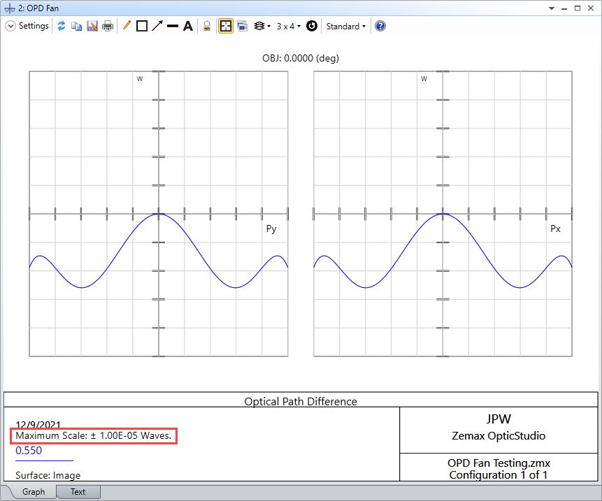
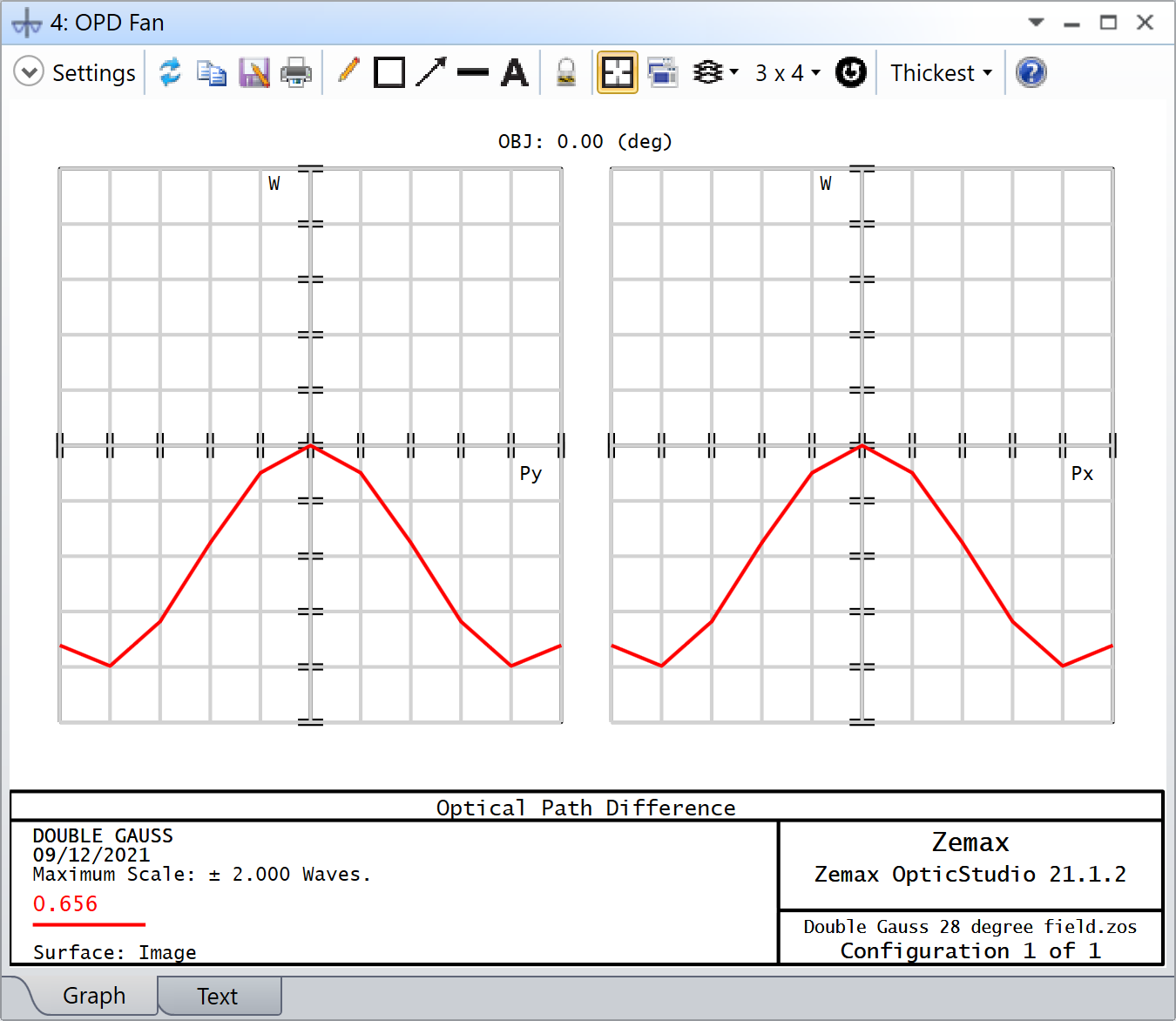
I notice that your OPD values are extremely small, which is likely the root cause of your problem. If I replicate your situation, here’s the corresponding OPD Fan:
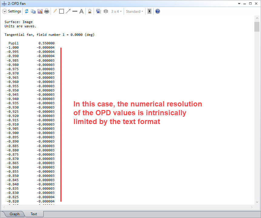
However, the values reported in the Text window have limited numerical precision.
Here I’ve used 200 rays to increase sampling resolution, but if I simply cut-and-paste these values into Matlab and plot them, the result is similar to what you find.
The stair-step nature of the plot is simply the result of high sampling with limited precision. Unfortunately, I don’t think there is any way to change the precision of the values reported in the Text Window (although I could be wrong and just don’t know where the control is located).
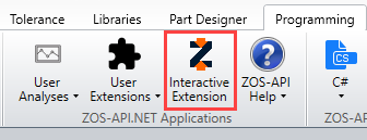
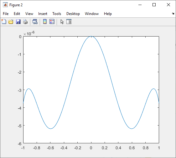
However, OpticStudio internally uses double-precision values, and these data can be readily extracted from the analysis window using ZOS-API. I prefer to use Matlab for the interface and work in interactive mode:
After clicking on “Interactive Extension” to start the process, entering the following code in an open Matlab shell window establishes communication, grabs the desired data and plots it.
% **** data for tangential OPD fan **** % link to existing OPD Fan analysis window opd_dbl = TheSystem.Analyses.Get_AnalysisAtIndex(2); data = opd_dbl.GetResults().DataSeries(1); % get first data series x = data.XData.Data.double; y = data.YData.Data.double; figure, plot(x,y)
I think the OPD in OpticStudio uses linear interpolation between the points. If you reduce the number of rays to the absolute minimum, which is 5, you get a plot like so (in the Double-Gauss example):
The more rays you trace, the smoother it will look, but since it is the result of a linear interpolation, it never is trully continuous.
I haven’t programmed with MATLAB in a long time, but it seems you have made a sort of bar plot somehow. It looks like it uses a nearest-neighbour interpolation. Basically, at Py = 0, you have a 0 OPD, but in your plot it gets propagated between Py = -0.1 and Py = 0.1. Then, it jumps to the next point Py = 0.2, where the OPD is -1. What OpticStudio does is it linearly moves the OPD from 0 to -1 between Py = 0 and Py = 0.2.
There are two things you should do, imo. First, if computation speed permits, increase the number of rays, to get more samples. Second, do a linear interpolation between the points as opposed to a nearest-neighbour interpolation. It is always a good idea to rely on more points, as opposed to an interpolation scheme. Let me know if these things aren’t clear to you.
If you could share your code, we could have a look at it and tell you how to correct it. I thought MATLAB plot function was interpolating by default with something more elaborated than nearest neighbour, is that the function which you used?
I notice that your OPD values are extremely small, which is likely the root cause of your problem. If I replicate your situation, here’s the corresponding OPD Fan:
However, the values reported in the Text window have limited numerical precision.
Here I’ve used 200 rays to increase sampling resolution, but if I simply cut-and-paste these values into Matlab and plot them, the result is similar to what you find.
The stair-step nature of the plot is simply the result of high sampling with limited precision. Unfortunately, I don’t think there is any way to change the precision of the values reported in the Text Window (although I could be wrong and just don’t know where the control is located).
However, OpticStudio internally uses double-precision values, and these data can be readily extracted from the analysis window using ZOS-API. I prefer to use Matlab for the interface and work in interactive mode:
After clicking on “Interactive Extension” to start the process, entering the following code in an open Matlab shell window establishes communication, grabs the desired data and plots it.
% **** data for tangential OPD fan **** % link to existing OPD Fan analysis window opd_dbl = TheSystem.Analyses.Get_AnalysisAtIndex(2); data = opd_dbl.GetResults().DataSeries(1); % get first data series x = data.XData.Data.double; y = data.YData.Data.double; figure, plot(x,y)
Thank you for your reply. I really appericate the help. I have not yet worked with the matlab extension, so I first give it a try. I’ll come back to your answer as soon as I have tested it!
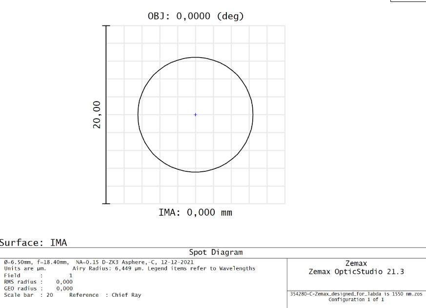
Just one last quick comment. As you may know, when the OPD takes on such tiny values, the exact shape of the fan isn’t particularly important because the lens system will be very deep into the diffraction-limited regime.
Thank you for your additional information. In all honesty, I was not fully aware of this, but I should have. Thank you for making me aware. Indeed, looking at the spot diagram, where the Airy disk radius is also plotted, the plotted blue dot, does not resemble any physical meaning anymore.
Just for some background, I was optimizing a surface (conic constant and 4th order term of the zag formula) of a collimating lens for a specific wavelength (1550 nm) such that the collimating-lens became a diffraction-limited system.