Solved

extended source encircled energy

  • 11 January 2021
  • 12 replies
  • 1416 views

Hello,


Could you tell me how the extended source encircled energy calculation works? And also how the 'multiply by diffraction limit' applies to the calculation?  


Also, how does the 'multiply by diffraction limit' compare to the calculation: 'diffraction encircled energy'?


I calculate both and I am wondering why they are different.


thank you

icon

Best answer by Angel Morales 11 January 2021, 23:51

View original

12 replies

Userlevel 5
Badge +1

Hi John!


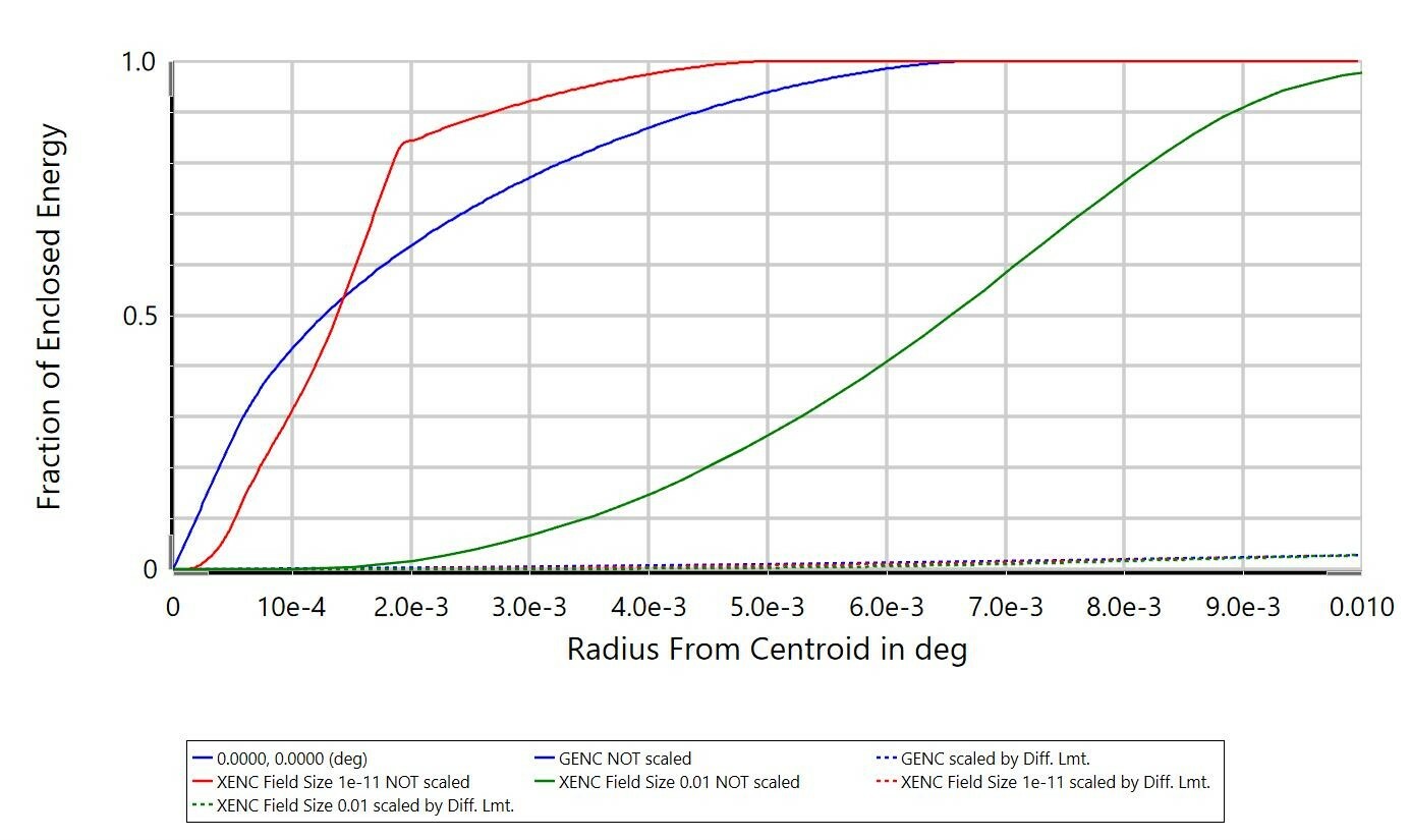
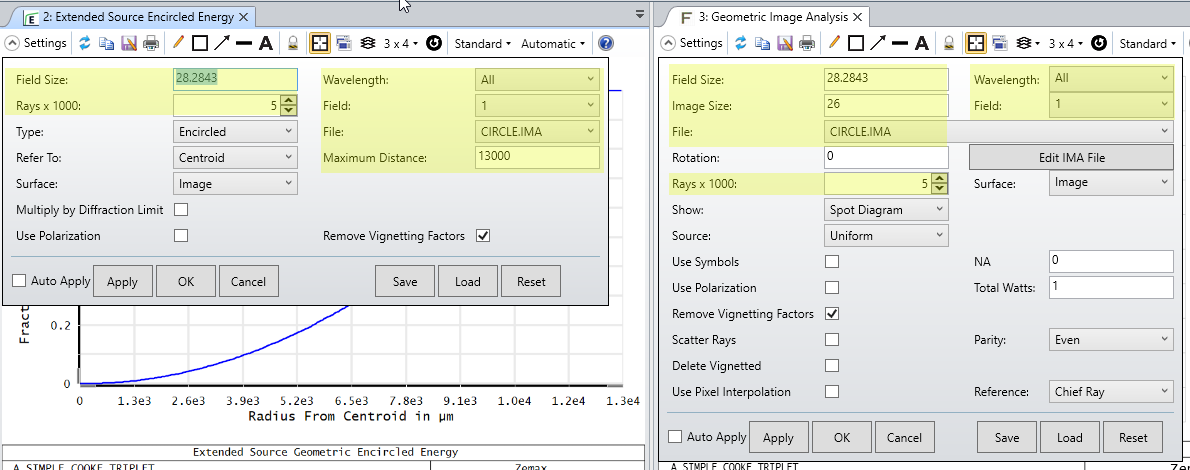
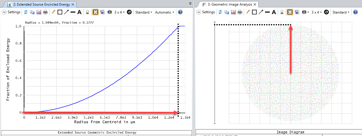
The Extended Source Encircled Energy analysis obtains results in a very similar manner to the Geometric Image Analysis tool. In both, you effectively select an IMA file for OpticStudio to generate rays from. You specify the size of the IMA file in object space and what field point the file is centered on. The difference is that Geometric Image Analysis will show the simulated image after tracing rays through your optical system, whereas the Extended Source Encircled Energy reports the fraction of energy that is arriving on your image plane as you go away from the centroid (or other reference point) of the simulated image:


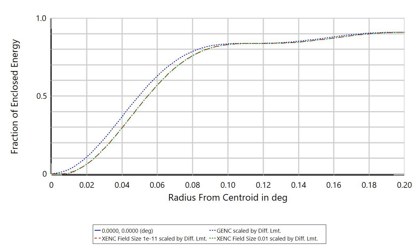
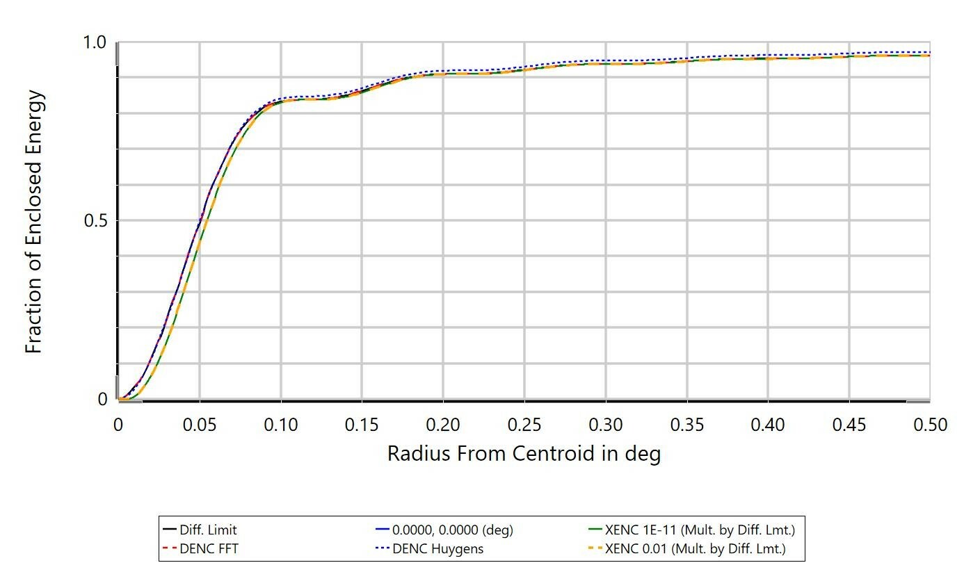
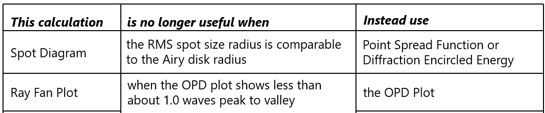
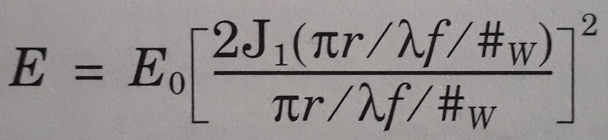
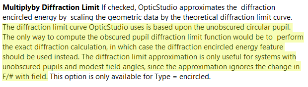
The differences between Extended Source Encircled Energy and the diffraction-based computation Diffraction Encircled Energy may come down to the optical system itself. In the Help Files, there is some discussion on the applicability of the 'Multiply by Diffraction Limit' setting (from 'The Analyze Tab (sequential ui mode) > Image Quality Group > Enclosed Energy > Extended Source'):


Let us know if you have any further questions here, or if anything else needs clarifying!


~ Angel

Userlevel 3
Badge

I have the same question. I understand how the Extended Source Encircled Energy works like the Geometric Image Analysis.  But the question is really about the details on how the 'Diffraction Limit' is defined and applied in these different analyses.


Let's abbreviate the names of the analyses as 'Extended Source Encircled Energy' = XENC and 'Diffraction Encircled Energy' = DENC. (like the corresponding merit function operands used to calculate the distances to the e.g. radius to a specific encircled fraction, which is what I want to find)


[Geometric Encircled Energy GENC appears to work the same as XENC except only for point source objects; i.e. I think that the answer for XENC should apply to GENC, too.]


Please elaborate a bit on the 'diffraction limit' and how it is calculated.  The User Manual/Help File entry 'Multiply by Diffraction Limit' quoted above by Angel from the section on XENC refers to a 'diffraction limit curve' based on a circular pupil.  [We'll keep this discussion confined to a circular pupil, and 'encircled' energy for now!]


Is there a separate 'diffraction limit' calculated for each point along the XENC curve (i.e. for each abscissa, corresponding to each point on the x axis of either radial spot size or, in afocal mode, angular radius)?  If so, could you explain how each point on the Diffraction Limit Curve is calculated?


The 'Multiply by Diffraction Limit' terse checkbox label in XENC initially made me think that in XENC, there was a SINGLE 'diffraction limit' constant number used to multiply the entire geometrically-calculated curve.  By analogy, the 'Show Diffraction Limit' checkbox in the 'RMS vs. Field' analysis appears to do this...drawing a horizontal line at '1.22 times the Working F/# on-axis times the primary wavelength'.  And the Airy Disk on Spot Diagrams needs to use this single number.


But reading more about XENC, DENC, and MTF calculations, it sounds like there is a different diffraction-limited number calculated at each point along the curve for these analyses.  The entry in the User Manual on the definition of 'Diffraction Limited' has a bit more detail on how perhaps setting OPD to zero is used, but I couldn't follow that completely.


DENC sounds like it is doing a more detailed 'diffraction limit' calculation than XENC, for every point along the curve, and I would always choose 'Use Huygens PSF' since it seems plenty fast. What's the alternative to using the Huygens PSF for the calculation?


Anyway, I don't fully understand sampling and proper use of DENC and when to choose it instead of XENC (based on the system parameters).  I will probably confidentially send you an actual system under a support ticket for advice on which analysis should provide the most realistic calculations for our system.  And to compare the differences between the calculated XENC and DENC for that specific system...if they differ much at all.


Is one of DENC and XENC (or GENC) better for a system that is close to diffraction-limited, and one better for a system that is far from diffraction limited?  Or is DENC always better than GENC--with XENC like a form of GENC necessary to accommodate an extended source?  Is an extended-source version of DENC possible (but not yet supported)?  How about off-axis systems like one including an off-axis parabola?


-- Greg

Userlevel 3
Badge

I've answered my question on Huygens PSF vs what...should have read the DENC Discussion section in the User Manual more carefully, where right at the beginning it says,


'See the discussion sections of the FFT and Huygens PSF. Those comments also apply to this feature.'


So I'll have to study the sections on FFT PSF and Huygens PSF. I think they also apply to MTF calculations.


====


I expect to find that Extended Source Enclosed Energy (XENC) should give the same result or curve as Geometric Encircled Energy (GENC) if the 'Field Size' parameter in the XENC settings is set to a relatively TINY number (e.g. 1e-07).  I.e., if the Extended Source size is set so small that it looks like a point source.


Right?

Userlevel 6
Badge +2

Hello Greg


Sorry for not replying to your previous message but I am glad that you found the information.


Regarding to your question, XENC is giving the energy for a full source: so basically field points sampled to represent a source. GENC gives the encircled energy for one field at a time.


So yes if the field size is very small, we should expect the results to be the same if not close.


Do not hesitate if you have any further questions.


Sandrine

Userlevel 3
Badge

Thank you, Sandrine, for your reply posted a week ago.  I still have some of the same questions that were in my previous posts; the only one I had actually answered myself before my latest post was, 'What's the alternative to using the Huygens PSF for the calculation?' [Answer: FFT PSF]


I still have the questions as to which one of DENC or XENC (probably not GENC) is the 'best' (likely to provide the most accurate result) for my system, which I will share privately.


But in the past week, I have done multiple simulations and overlay plots comparing the 3 analyses that I will share in upcoming posts, as others might also find them interesting.


One question was how the Diffraction Limit curve is calculated for 'Show Diffraction Limit' (available in DENC, but not GENC or XENC), or 'Mutliply by Diffraction Limit' (available in GENC and XENC). My guess (supported by overlay plots) is that this is a point-by-point curve generated using the FFT PSF (not the Huygens PSF).  Right?  And that this curve is multiplied point-by-point for GENC and XENC curves when 'Multiply by Diffraction Limit' (labeled in the analysis plot window as 'scaled by diffraction limit').  Right?


As for XENC vs GENC, you confirmed my intuition that the results SHOULD be the same if the field size is set very small for XENC (i.e., approximating a point source).  I have found that they ARE NOT, EITHER for very small radii well below the diffraction limit (with 'Multiply by Diffraction Limit' unchecked) OR for large radii with Multiply by Diffraction Limit checked.  I'll share my curves showing this in my next (separate) post to this thread.


If the XENC curve for a point source looks different from the GENC curve, then there must be some difference in how these analyses are calculated. (a different algorithm? different assumptions that are not stated? or code errors?)


-- Greg

Userlevel 3
Badge

Re: XENC vs GENC.  Here are the two overlay plots I just mentioned comparing the calculated curves.


I am not attaching the model, because it is confidential. But I can say that it is very simple, having just a Paraxial XY surface and a tilted, very small curvature, spherical mirror. The analyses are performed in afocal image space, so the spot radius results are angular (in degrees) instead of in lens units such as micrometers. The system is small in scale, with diameters, thicknesses, and radii on the order of 1 mm. There is a tilted element.  But there is only one field point ON AXIS (0, 0), and I checked that there is NO vignetting, so that the Vignetting Diagram shows that the fraction of unvignetted rays is 100%, and ALL of the GENC, XENC, and DENC curves approach a Fraction of Encircled Energy = 1.0 at large radii.


The first plot is 'EncircledEnergy_GENC-XENC_small_radius.jpg' showing XENC (red curve) vs GENC (blue curve) without Mutliply by Diffraction Limit checked. A point source in XENC is modeled by setting Field Size = 1e-11. (a 10 um field size, i.e. 0.01, is also shown in the green curve and behaves as expected). One can see that although these results are not physical (way below diffraction limit), the curves are different shapes, meaning they are calculated differently somehow.


[Note that the '0.0000, 0.0000 (deg)' blue line corresponding to the 'host' plot for the overly is not used...can't turn it off in the legend; so the displayed blue line is shown in the legend as 'GENC NOT scaled'.]


The dotted lines in that previous 'small radius' plot lie close to the abscissa (x axis) because they are the 'scaled by Diff. Lmt.' curves that only increase at much larger radii.


The second plot here is for larger (physically significant) radii, comparing the plots when scaled by the diffraction limit ('Multiply by Diffraction Limit' checked), and I gave it the file name 'EncircledEnergy_GENC-XENC_MultByDiff.jpg'


Again, it can be seen that the GENC curve (scaled by Diff. Lmt.) in the blue dots is NOT coincident with either of the XENC curves scaled by Diff. Lmt., although the XENC curves, corresponding to Field Size 1e-11 (red dashes) and Field Size 0.01 (green dots) lie exactly on each other. I think this shows that a 10 um Field Size is plenty small enough already to have no effect on a diffraction-limited system of this size. (again, the '0.0000, 0.0000' curve is not used)


It is not surprising that all of these curves converge at large radii to the same Fraction of Encircled Energy = 1.0.  What matters for us is what number the analyses calculate for a spot radius (angular in our case) for which a given fraction, e.g. 90%, of encircled energy is specified (as in the XENC merit function operand, given e.g. Frac = 0.9)... And which is the most realistic/correct number from these alternative XENC, GENC, and DENC analyses.


-- Greg

Userlevel 3
Badge

Re: DENC vs XENC.


Here is an overlay plot comparing DENC to XENC (multiplied/scaled by 'diffraction limit') for the same system.


Again, our question is which of the analyses produces the most believable estimate for the radius at which a given fraction of encircled energy is achieved. (I will be using e.g. the XENC merit function operand with e.g. a Frac = 0.9 to return the radius at which 90% of the energy is encircled.)


And why do these calculations give differing results?  I think this is pretty much a diffraction-limited system, and as I said, there is no vignetting.


Below is the plot, to which I gave the file name, 'EncircledEnergy_DENC-XENCscaled_comparison.jpg'*


We see that the 'Diff. Limit' (solid black) curve lies on top of the 'DENC FFT' (red dashes) curve, which is what led me to believe (and ask in my post before last) that the Diffraction Limit curve is calculated using the FFT PSF. Likewise (as I also guessed above) I'm thinking that the FFT PSF is used to calculate a Diffraction Limit curve that is multiplied point-by-point with the GENC and XENC curves when 'Multiply by Diffraction Limit' is checked in the GENC and XENC analysis window settings.


The XENC curves for a tiny source (Field Size = 1E-11, green curve) and for a merely 'very small' source (Field Size = 0.01, yellow dashes) lie right on top of each other, but are shifted (at small radii) to the right of the 'Diff. Limit/DENC FFT' curve, meaning that XENC calculates a larger radius for the same encircled energy (or equivalently, a smaller fraction of encircled energy for the same radius) than DENC. At 0.10 deg, corresponding to an encircle fraction of about 83%, those curves merge together, though for all greater radii.  Why are DENC and XENC results different at small radii?  Since the two XENC curves (for different source sizes) are the SAME at small radii, I can't attribute the difference of XENC from DENC to the size of the extended source.


Finally, comparing Huygens PSF vs FFT PSF in the DENC analysis:

'DENC Huygens' (checking the box 'Use Huygens PSF') results in the blue dotted curve, which starts out lying on top of the 'DENC FFT' red dashed curve and between 0.05 and 0.10 deg, remains higher than DENC FFT -- and 'Diff. Limit' for all greater radii.  I have found this result consistently, i.e., Huygens PSF predicts a higher encircled energy for a given radius, or equivalently, a smaller radius spot for the same fraction of encircled energy, than the FFT PSF. By 'consistently,' I believe that this discrepancy is NOT due to under-sampling the pupil...the curves shown were generated using Pupil Sampling = 128x128 (higher than default 64x64), and remain smooth(er) and offset as shown for higher settings of Pupil Sampling.  Can anybody explain this?


-- Greg


*Don't look for the '0.0000, 0.0000 (deg)' curve (which would be a solid blue line), because although it would be the main curve in the 'host' DENC analysis window, I suppressed it by unchecking it in the 'Legend Checkboxes' (not shown). I only showed the overlaid curves from different windows, and the black 'Diff. Limit' curve supplied in the host analysis window, because I could edit or use the descriptions of them in the legend. The name/legend text for the main curve in the overlay plot apparently can't be edited!  FEATURE REQUEST!!

Userlevel 6
Badge +2

Hi Greg


First about the diffraction limit:


- If you are calculating the enclosed energy using geometric rays, then the result can become overly optimistic when the system starts to approach the diffraction limit. Rays can give you a perfect point whereas diffraction will tell you are limited by the Airy disk. So this is why for geometric calculation there is an option that provides a compromise. It allows to multiply the result by the theoretical limit value of diffraction so that the result can not be better than a perfect limited diffraction system.


- But if you are in a close to diffraction limited system, I would just use diffraction calculations as they will be the most accurate. In the diffraction calculation, you will get a Diffraction Limit curve showing the diffraction limit. This is basically the result for a Bessel function. 


Now about the comparison between GENC and XENC:


- I have worked on the Cooke triplet sample file: '\Zemax\Samples\Sequential\Objectives\Cooke 40 degree field.zmx'. As you can see, the results for GENC and XENC are equivalent for the same field. Equivalent but not identical.

And the reason for this is that we simply don't use the same method to calculate them.

In the case of GENC, rays start from a field point and aim at the pupil. The number of rays used by that analysis is given by the pupil sampling.

In the case of XENX, we select a certain number of rays on the image to properly sample the pixels of the 'bitmap'. Then we send those rays. It is equivalent to the Geometric Image Analysis in the way it works. In the help file under The Analyze Tab (sequential ui mode) > Image Quality Group > Extended Scene Analysis > Geometric Image Analysis, there is a section that explain how rays are chosen:


If you have a specific file, we would be happy to have a look at it. I feel it is much easier to discuss on a specific case.


Sandrine

Userlevel 3
Badge

Sandrine,


Thanks so much for looking at all this detailed material and for replying so quickly!


I am satisfied why the curves generated by XENC and GENC are not the same, now that you have confirmed that they do use a different method to generate the rays used in the calculation. That explains the first 2 overlay plots in my posts above, both for the (unphysical) small radii (unscaled) shown in the first plot, and for the 'Mutliplied by Diffraction Limit' curves in the second plot.


And thank you for running and sharing the XENC vs GENC comparison using the publicly-available Cooke Triplet model.  I have looked at it and can see how the XENC and GENC curves change only slightly (in the direction expected, i.e. wider spot) when 'Multiply by Diffraction Limit' is checked.


I suppose this (and the fact that there are many rays in the spot diagram outside of the Airy disk) means that the Cooke Triplet system is FAR from diffraction-limited.  And therefore these ray-based encircled energy plots GENC and XENC provide valid estimates (if not identical) in your example.


*** Can you suggest a simple test (some optical path difference operand value calculation, system data report, whatever) to use for a quick check as to whether the system is 'close to diffraction limited' for the purposes of these encircled energy plots?  And hence suggests that DENC is the best choice?  Kind of a go/no-go check?


Can you confirm that the calculation used to generate the 'Show Diffraction Limit' curve from DENC is the FFT PSF?


And that the 'Multiply by Diffraction Limit' option in XENC and GENC use that same calculation as for the DENC 'Show Diffraction Limit' curve, together with a point-by-point multiplication (convolution?) with the geometric ray-calculated curves?


Do you have any idea why encircled energy curves calculated using the Huygens PSF would be a bit narrower/higher (at larger radii) than those calculated using the 'default' (FFT PSF) setting?


-- Greg

Userlevel 6
Badge +2

Hi Greg


In our training slides, here is how we define diffraction-limited:


  • The Strehl Ratio is greater than 0.8 which corresponds to the RMS wavefront being less than λ/14.

  • A traditional criterion is the peak-to valley OPD is less than 1/4 of a wave but this is a weaker criterion than the RMS.


Remember, there is no 'hard edge' where the lens is suddenly diffraction limited. It is just a threshold where reductions in the aberrations will not yield a significant improvement. So here is a table that gives some indications on which calculation to use:


For the 'Show Diffraction Limit' curve in the DENC, we simply use the Bessel function. 


So in the 'Field Guide of Geometrical Optics', you can read that the energy of an aberration free optical system follows:


where r is the radial coordinate, J1 is a Bessel function and f/#w is the image space working F#.


The Multiply by Diffraction Limit option is only available for XENC and GENC. Because there is a risk to get a better result that an aberration free system if we don't take into account aberration. For DENC, we do not have that option as we take into account diffraction in the calculation. So we only display what a perfect system would be with the option Show Diffraction Limit. 


For the difference between Huygens and FFT, I don't know why your results are different but the calculation of both are different and also the assumptions. We always say to trust the Huygens because it contains less assumptions. Both methods are using the scalar diffraction theory (so the beam should not be too fast). The FFT makes a FT of the pupil. It assumes the image is in the far field and the chief ray is perpendicular to the image. The Huygens is done at the image. Check our help file for a detailed description. 


Sandrine

I have an afocal system as well and I want to find the encircled energy on a circular detector.

I’m using the extended source geometric encircled energy with a field size of 0.01 and the circle.ima source. 

I want to know how much energy is in the radius of the detector. Since the output is mr from the centroid, how do I convert that to um? How far is the extended source?


Thanks!

Userlevel 6
Badge +2

Hi Arlette,

I think you can simply untick Afocal Image Space to work again in distance instead of angles.

The Extended Source is defined by the Field Size setting. In the help files, it says that the Field Size setting defines the full width of the square image file in field coordinates. So if you selected circle.ima, it means that you have an extended source with a diameter of 0.01. The units are the same as your field coordinates.

Reply