Hi everyone!

If you have ever tried to find a good reference for modeling a beam splitter in Zemax, you have probably noticed that most examples either go the Non-Sequential mode, which means losing access to aberration metrics, OPD, MTF and all the sequential analysis tools we rely on, or they use Sequential mode but with a multi-configuration setup, which works but can get unnecessarily complicated depending on what you are trying to simulate.

After going through that myself, I put together this guide in case it helps anyone who runs into the same situation, since getting this right can be trickier than it looks. The goal is to show a simpler path: a non-polarizing beam splitter modeled entirely in Sequential mode, in a single configuration. No mode switching, no extra configurations. Just a clean sequential system that still gives you full access to all the analysis tools.

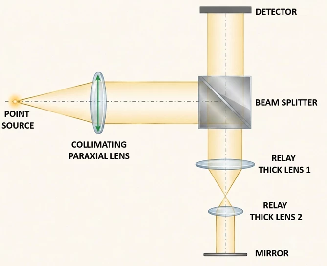
To keep things concrete, the system I will use as an example is based on this layout, which is pretty close to what you would find in a surface metrology setup like a Fizeau interferometer:

Step 1

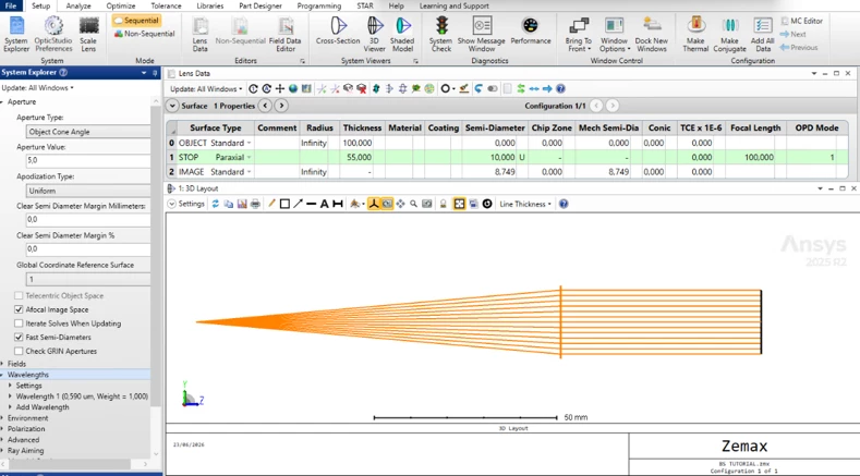
The first thing we need to do is define how light enters the system. In this case I used a paraxial lens to collimate the beam from a point source, but if you prefer a simpler approach you can just place the object at infinity and define the aperture as an entrance pupil diameter. Both work fine for what we are building here.

For this example the setup looks like this: a point source at 100 mm from a paraxial lens with a focal length of 100 mm, which gives us a clean collimated beam at the output.

Step 2

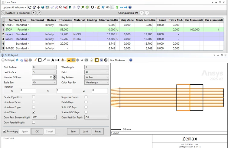
Now we start modeling the beam splitter itself. We are using a 1 inch cube (25.4 mm per side), so we split it into two equal halves of 12.7 mm each, with the beam splitting interface sitting right in the middle. In the Lens Data Editor this translates to two Standard surfaces with N-BK7 glass and a thickness of 12.7 mm each, giving us the full cube when combined (surfaces 2 and 3). One small tip for this stage: check the Hide X Bars option in the 3D Layout settings. It just makes the visualization cleaner while you are building the geometry, though you can turn it off later once everything is in place.

Step 3

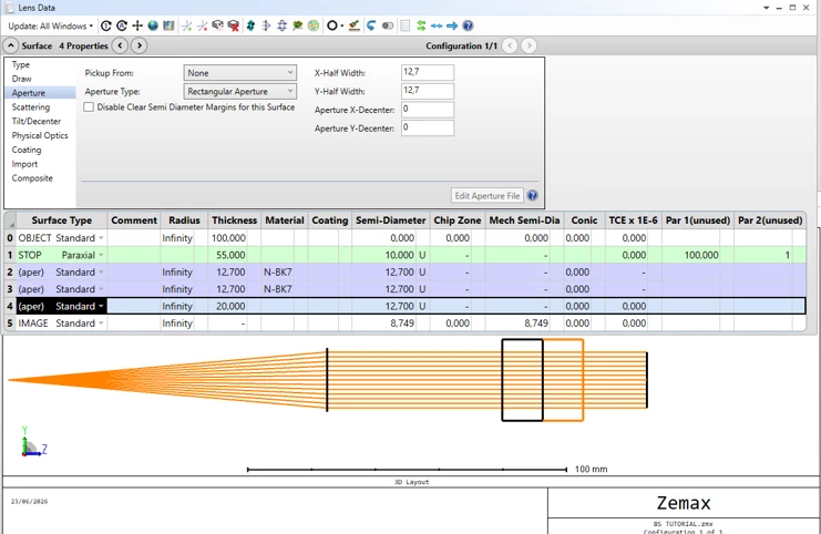
At this point the beam splitter surfaces have floating apertures, which means Zemax is treating them as circular by default because of the light beam. If you look at the 3D Layout you will see a cylinder instead of a cube, which is not what we want. To fix this, go into the surface properties for each of the beam splitter surfaces and change the aperture type to Rectangular Aperture, setting both X and Y half-widths to 12.7 mm. Do this for all the surfaces that make up the cube and you will get the correct square cross section in the layout. One thing worth noting from this point on: the Cross Section view will no longer be available for this system. From here you will need to use the 3D Layout to visualize the geometry, so keep that in mind as we add more elements in the next steps.

Step 4

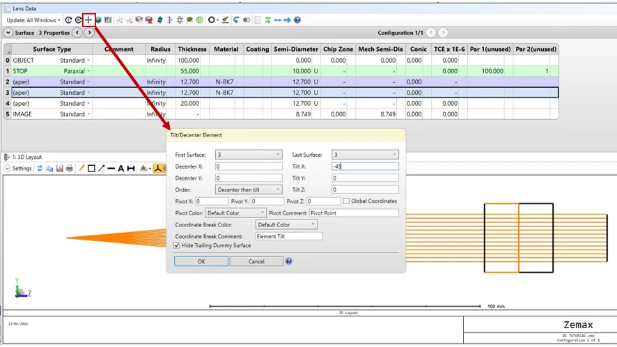
Now we need to tilt the central surface so it actually acts as a beam splitter. To do this, select surface 3 and open the Tilt/Decenter Element tool. Set Tilt X to -45 degrees and make sure the option Hide Trailing Dummy Surface is checked to keep the Lens Data Editor clean. This will automatically insert the two Coordinate Break surfaces around surface 3, handling the tilt and the return for you. At this point the geometry is in place and the splitting surface is correctly oriented at 45 degrees inside the cube.

Step 5

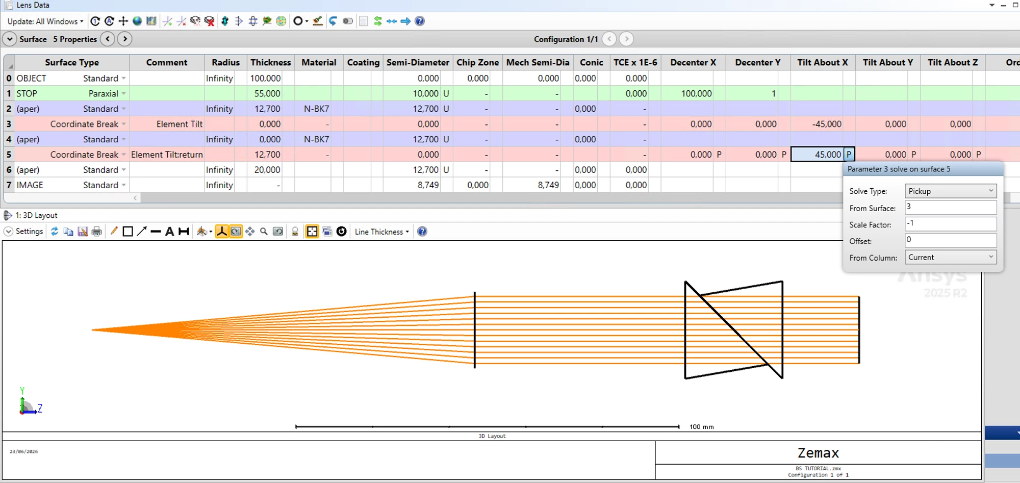
After clicking OK, Zemax automatically inserts two Coordinate Break surfaces around the tilted surface. You can see in the Lens Data Editor that surface 3 now holds the -45 degree tilt and surface 5 is the return CB with a +45 degree pickup from surface 3 and a scale factor of -1, which is not what we want but we will modify it later. One thing to verify here: surface 4 should have a thickness of 0, and the 12.7 mm thickness should sit on the return Coordinate Break at surface 5. If the thickness ended up on surface 4 instead, just move it over manually. At this point you can already see in the 3D Layout that the cube has the diagonal interface correctly placed at 45 degrees inside it, even though the rays are still passing straight through since we have not assigned the mirror behavior yet.

Step 6

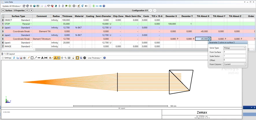
By default, the return Coordinate Break is set with a scale factor of -1, which simply undoes the tilt and brings the optical axis back to its original direction. But that is not what we want here. We need the optical axis to rotate 90 degrees total, which means the return CB should apply another -45 degrees instead of canceling the first one.

To do this, open the pickup solve on surface 5 Tilt About X and change the scale factor from -1 to 1. This way both Coordinate Breaks apply -45 degrees each, adding up to a full 90 degree rotation of the optical axis, which is exactly what a beam splitter redirecting light downward would do.

Step 7

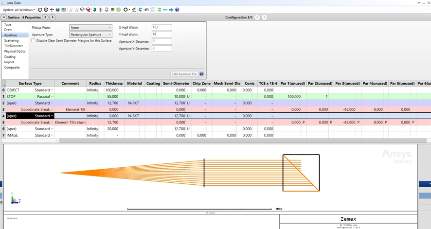
Since the beam splitting surface is tilted 45 degrees inside the cube, its physical footprint is no longer square. The diagonal interface is longer along one axis, so we need to account for that in the aperture definition.

Go into the properties of surface 4 and set the aperture to Rectangular, keeping the X half-width at 12.7 mm but setting the Y half-width to 12.7 × √2 ≈ 18 mm. This correctly represents the elongated shape of the interface as seen from the tilted reference frame, and prevents OpticStudio from clipping rays that should be passing through the full aperture of the cube.

Step 8

Now we assign MIRROR as the material of surface 4. As soon as you do this you will see in the 3D Layout that the rays bend 90 degrees at the beam splitter, which is exactly the behavior we are looking for. However, there is an important side effect: after a reflection in sequential mode, the direction of propagation flips, so all the thicknesses that follow the mirror surface need to change sign to propagate correctly. In this case the return Coordinate Break at surface 5 changes from 12.7 to -12.7 mm, and surface 6 from 20 to -20 mm. If you leave them positive, Zemax will trace the rays in the wrong direction. You can already see in the layout that the beam is now being redirected downward and converging, which confirms the geometry is working as expected.

Step 9

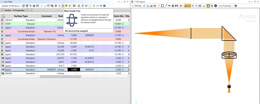
Now we add the relay lens group and a flat mirror at the end of the optical path, placed 7.5 mm from the last surface of the second relay lens. At this point you have two options to complete the return path. You can manually re-enter the relay lens surfaces in reverse order so the beam traces back through them, or you can use the built-in Make Double Pass tool, which automates exactly that. Select it and set the reflection at surface 13, which is the mirror, and Zemax will generate the return pass for you automatically with corresponding pick-ups.

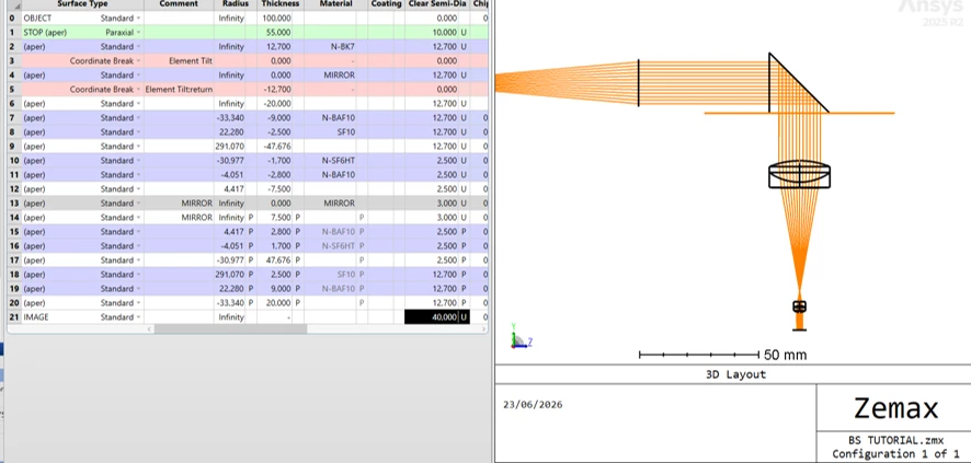
The 3D Layout now shows the full system working as intended: the collimated beam enters horizontally, gets redirected 90 degrees downward by the beam splitter, passes through both relay lenses, hits the mirror, and comes back up through the same lenses toward the image plane.

Step 10

After applying Make Double Pass, Zemax duplicates the entire system after the mirror reflection with the correct signs. However, we only need the two relay doublets on the return path, so delete everything else that was generated beyond them.

Once cleaned up, you will notice that the last surface in the system is the bottom face of the beam splitter cube. To confirm visually that the beam is arriving at the right place, increase the size of the image surface temporarily. This makes it easy to see in the 3D Layout that the rays are correctly propagating back up through the relay lenses and reaching the bottom of the cube, right where the beam splitter interface sits.

Step 11

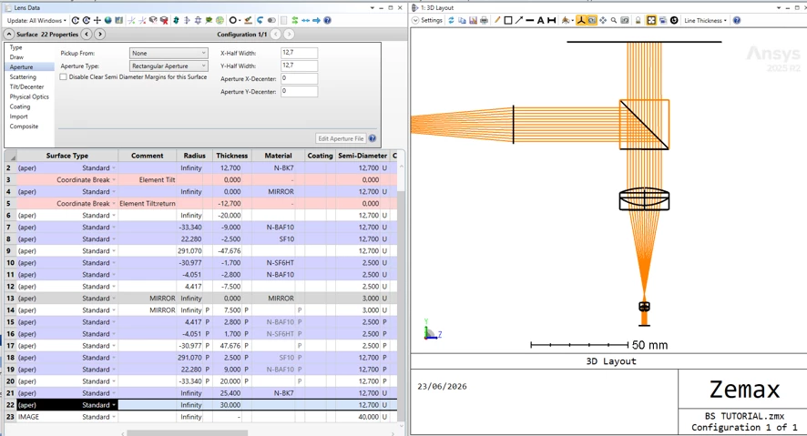
To finish the system, we add the upper half of the beam splitter cube as a simple transmission block. From the last surface, insert a N-BK7 block with a thickness of 25.4 mm and rectangular apertures of 12.7 mm in both X and Y. There is no splitting interface here, just glass in transmission, since the beam is now traveling straight up toward the detector.

One thing worth noticing at this stage: after the mirror reflection earlier the thicknesses turned negative, but now that the beam has reflected again at the beam splitter surface and is propagating upward, the thicknesses go back to being positive. This sign behavior is something to keep an eye on whenever you have multiple reflections in a sequential system, as getting it wrong will cause the ray trace to break.

The 3D Layout now shows the complete system, with the beam traveling from the source, through the beam splitter, down through the relay lenses, bouncing off the mirror, coming back up through the relay lenses, passing through the upper cube, and reaching the detector.

Final note

With this, we have a fully working beam splitter in a single sequential configuration for a double pass system, which means we can run optimizations and evaluate performance metrics without having to manage multiple configurations or switch modes.

If you plan to do tolerancing on this system, the recommended approach in my opinion is to add Coordinate Breaks at the relevant surfaces and define the pivot points for decenters and tip-tilt where physically meaningful. From there, use TPAR operands to perturb the Lens Data parameters and set up pickup solves on the duplicated surfaces that appear after the reflection, so that any perturbation applied to an element on the way down is automatically mirrored on its counterpart on the way back up. Without those pickups, you would end up tolerancing both passes independently, which does not reflect how the real system behaves.

Hope it helps!

Jesús