OpticStudio supports Q-type aspheres. Type 0 indicates Qbfs polynomials, and Type 1 indicates Qcon polynomials. The functional forms of the Q-type polynomials are fairly complex due to the requirement that the polynomials be orthonormal for a circular aperture. Occasionally, it is convenient to know the functional form of the polynomials for testing and comparison purposes.
Below, we list the first 10 Qbfs polynomials, and also share how to calculate them in the Mathematica file GenerateQbfsPolynomials.nb. The .nb files for Mathematica can be used by downloading the free Wolfram Player: https://www.wolfram.com/player/.
Important equations for the Q-bfs polynomials
The equations used below come from Shape specification for axially symmetric optical surfaces, G.W. Forbes, Optics Express 5218, Vol. 15, No. 8, 16 Apr 2007. Forbes watned to find a function whose slopes are orthogonal. So the slope equations must obey:
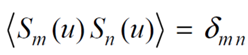
where u is the radial coordinate in the aperture of an optical surface, and dmn is the Kroeneker delta function, which is 1 when m = n and 0 for all other m and n.
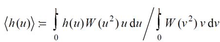
The weighted average indicated by the angled brackets above is defined as:
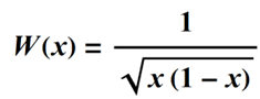
Forbes suggests choosing a weighting function that will enforce well-behaved slopes at the center and edge of an aperture, so that the weighting value is high when u = 0 and u = 1.
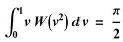
This choice of weighting gives a denominator in the weighted average of pi/2:
Forbes chooses the slopes as a set of general polynomial terms, which he calls the Q-bfs polynomials:
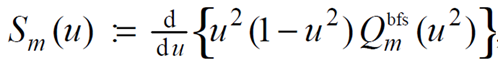
I'll just use a generic form for the the Q-bfs polynomials, initially, so:
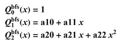
….etc.
And the orthogonality requirement gives systems of equations so that we can solve for the values of the coefficients.
For the first term, m = 0 and orthogonality condition is already satisfied:
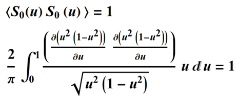
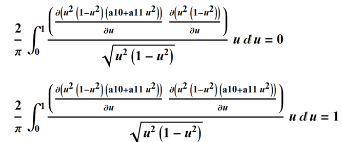
For m = 1, two conditions must be satisfied, so we have two equations and two unknowns coefficients:
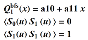
and in integral form using the definition of the weighted average above, the two equations are:
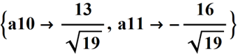
Solving the system of equations for a10 and a11 gives:
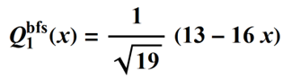
and the complete Qbfs polynomial is then:
The polynomials that follow can be calculated in the same way. For m = 2, we have three equations and three unknown coefficients:
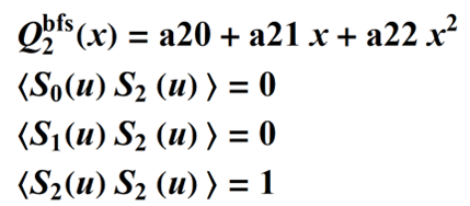
so we can solve for the coefficients to determine the complete polynomial, and so forth, for all the remaining polynomials.
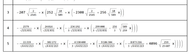
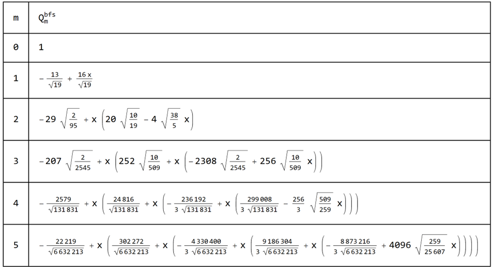
Listing of the Qbfs polynomials
The first 6 Qbfs polynomials are listed below.
Calculating the Qbfs polynomials
The attached Mathematica file, GenerateQbfsPolynomials.nb can be used to calculate any of the Qbfs polynomials. The .nb files for Mathematica can be used by downloading the free Wolfram Player: https://www.wolfram.com/player/. A .pdf version of the file is also attached to this article.