I have an optical system (refractive telescope + some lenses) to couple a laser beam into a single-mode fiber. I currently want to tolerance my system, so that the coupling efficiency does not drop below a threshold.
Currently, I use as a tolerancing criterion RMS Wavefront or RMS Spot Radius with a Paraxial Focus compensator. This works fine, but I have the feeling that those criteria don’t model the fiber coupling very well. Fiber coupling efficiency drops sharply if the focus spot moves from the center position, even if I compensate the shift with “Align Receiver to Chief Ray” feature in the Fiber Coupling tool.
I have tried to use the Merit function with a FICL operator, but this makes tolerancing really slow and FICL does not allow “Align Receiver to Chief Ray” I.e. sometime a smaller (better) RMS Spot Radius has a worse fiber coupling efficiency.
Maybe somebody has an idea, how to model fiber coupling more efficient to make the right decisions in the tolerancing process.
Many thanks Markus
Best answer by Jeff.Wilde
Hi Markus,
Ok, here’s what I would suggest. First, I think you should try to model your actual physical system as closely as possible. For example, using a tip/tilt mirror to steer the beam to the fiber center is different than having a perfectly on-axis beam and translating the fiber in (x,y). An off-axis beam will have different aberrations, and depending on where your tip/tilt mirror is positioned (relative to the front focal plane of the coupling lens system), it can produce varying chief ray angles at the fiber plane which can in turn affect coupling due to angular offsets. Second, you should ultimately use the FICL operand, but not as a first step because your random initial conditions will likely be far from the coupling peak, so FICL won’t generate enough of a signal to use for optimization (just as if you are in the lab looking at a fiber output signal on a power meter).
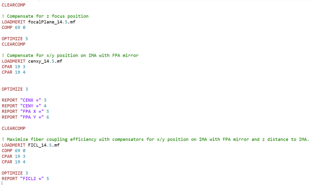
A better approach is to use a Tolerance Script and go through a sequence of steps as follows:
Clear all compensators.
Load a merit function that can be used for z-axis focus. Optimize to find the back focal plane location (at least roughly), using the back focal distance as a compensator, so that after optimization the fiber entrance face (located in the image plane) will reside at this approximate best focus. This can typically be done with just a few cycles of DLS, so in the interest of speed, just explicitly specify say 5 cycles. One important caveat. Construction of this merit function can be a little tricky because the spot size is varying slowly, and in the presence of aberrations the “best focal plane” isn’t particularly well defined. I’ve actually found that using an MTF value computed at a specific spatial frequency works reasonably well; however, this is something that takes a little investigation and experimentation for any given optical system.
Clear the z-axis compensator.
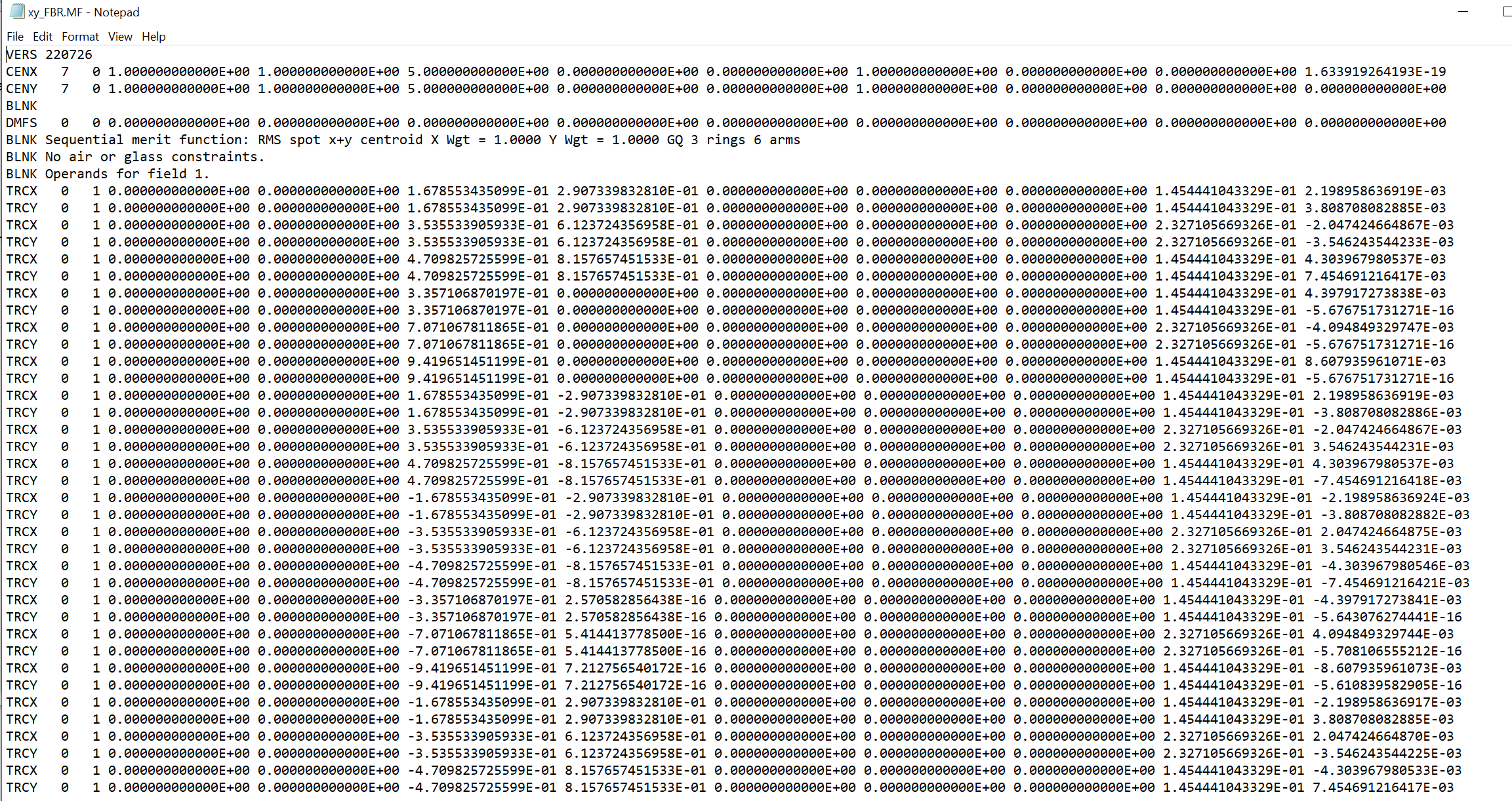
Load a merit function that can be used for finding the (x,y) centroid of the focused spot. This can easily be done using the CENX and CENY operands. Construct the merit function so that it drives the spot centroid to align with the (x,y) coordinates of your fiber center (assuming you include random fiber coordinates as part of your tolerance stack). Set the tip/tilt parameters of your mirror as compensators, and again perform a DLS optimization for a few cycles.
Clear the mirror adjustment compensators.
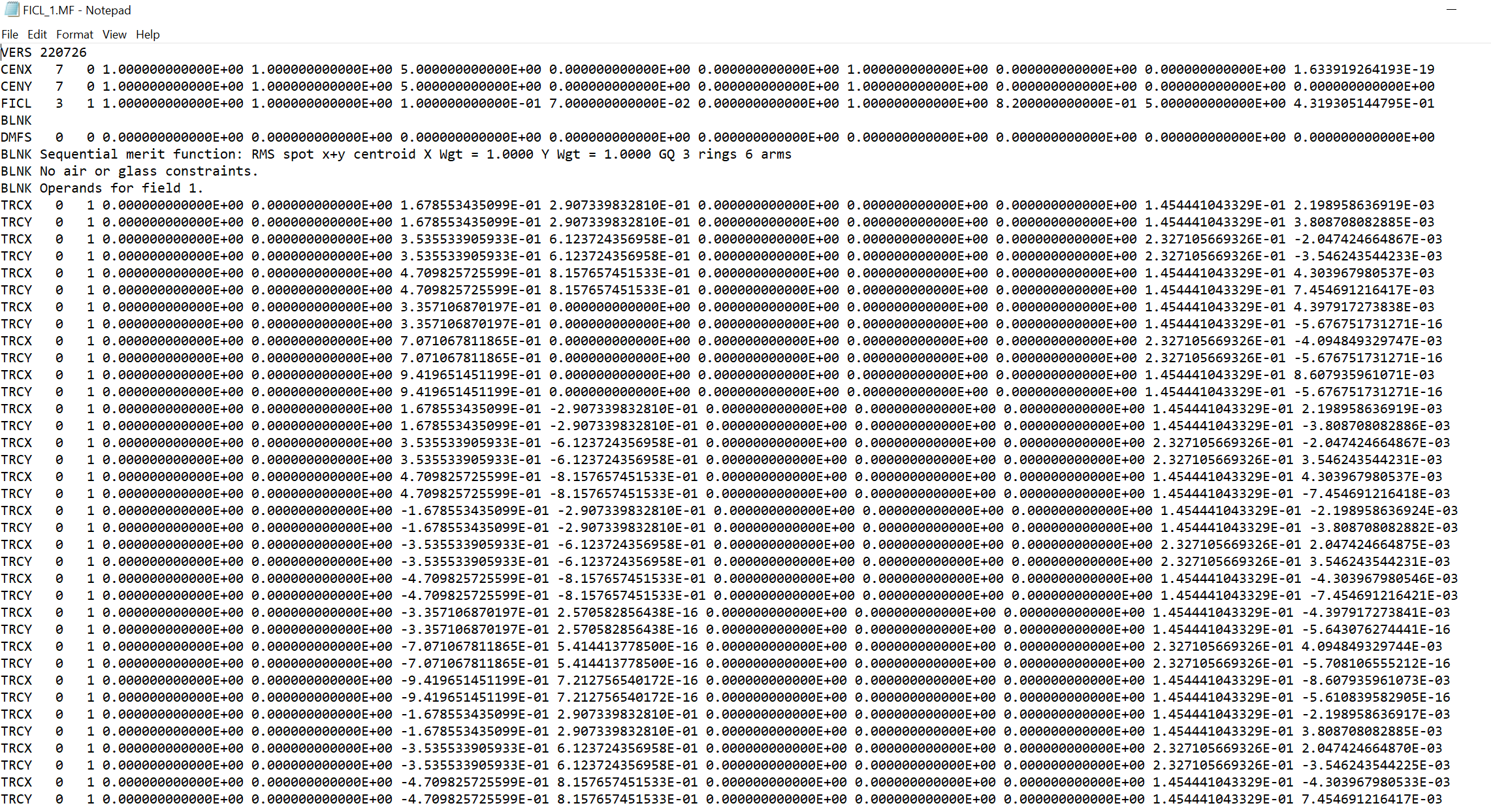
Load a merit function to compute fiber coupling using FICL. At this point, FICL should yield a reasonable value, at least large enough to use as an initial condition for optimization. In fact, from step (4) the spot centroid should already be centered on the fiber core. However, it’s good to dial-in the focus condition using FICL in order to peak-out the coupling efficiency. So, once again set the back focus (i.e., the fiber z-position) as a compensator and re-optimize, say using 3-5 cycles.
Clear the back-focus compensator.
Because in step (6) the fiber z-position is tweaked, this may also cause a slight (x,y) misalignment of the focused spot centroid relative to the fiber core center. So, as a last step, keep the fiber coupling merit function in place, but now again designate the mirror tip/tilt parameters as compensators and re-optimize.
Print out the compensator final values (i.e., the mirror tip/tilt values and the fiber z-position value) along with the value of the coupling efficiency.
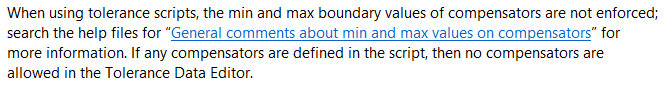
I don’t claim this particular set of steps is necessarily the best, it is just an approach that I have found useful in the sense that it is reasonably fast, robust and accurate, certainly much faster than simply using FICL from the start. One important last note, beware that when using a tolerance script, the min/max boundary values of compensators are ignored (and if even just one compensator is defined within the script, then all compensators must be defined within the script):
Therefore, it’s a good idea to include some operands in the various merit functions that limit the compensator ranges during optimization (simply to prevent some crazy run-away scenario that might drive the design in a nonsensical fashion).
First, one quick comment about "Align Receiver to Chief Ray." This option only translates the (x,y) position of the fiber center. It does not incorporate a tip/tilt of the fiber to match the chief ray angle. So even if the chief ray lands directly in the center of the fiber core, there could still be a reduction in coupling due to an angular mismatch (i.e., the focused cone of light is angularly offset from the fiber's acceptance cone).
Regarding tolerancing, I can make a few recommendations, but it would be helpful to understand more specifically what you are trying to accomplish.
For example, here are some possibilities:
1. The source is a fixed on-axis collimated Gaussian laser beam. The lens system has lens element fabrication errors plus element alignment errors that you wish the tolerance. The fiber is passively located at the nominal focal plane with some positional tolerances.
2. Same as (1), except now the fiber is actively aligned as the last step in the assembly process. This could be 2-axis alignment (x,y), 3-axis alignment (x,y,z), or 5-axis alignment (x,y,z,theta_x,theta_y).
3. Same as (1) or (2), but now you want to include some random perturbation of the source laser beam as part of the tolerance stack. This perturbation could be incorporated into the assembly process, or it could be investigated as a separate tolerance analysis post-assembly.
Does one of these scenarios match what you are trying to do?
Yes, I have a type 2 system, with a fixed on-axis collimated Gaussian laser beam as a source. In the real system, the fiber is fixed, but a tip-tilt mirror moves the focus spot to the fiber tip. We can move the z-position of the fiber tip manually as a compensator. I cannot correct theta_x/y, therefore I suspect that any operator like TEDX/Y or TETX/Y will also also create a tilt angle of the beam at the fiber tip, which I cannot correct and therefore will decrease efficiency. Of course RMS spot radius does not model this.
Ok, here’s what I would suggest. First, I think you should try to model your actual physical system as closely as possible. For example, using a tip/tilt mirror to steer the beam to the fiber center is different than having a perfectly on-axis beam and translating the fiber in (x,y). An off-axis beam will have different aberrations, and depending on where your tip/tilt mirror is positioned (relative to the front focal plane of the coupling lens system), it can produce varying chief ray angles at the fiber plane which can in turn affect coupling due to angular offsets. Second, you should ultimately use the FICL operand, but not as a first step because your random initial conditions will likely be far from the coupling peak, so FICL won’t generate enough of a signal to use for optimization (just as if you are in the lab looking at a fiber output signal on a power meter).
A better approach is to use a Tolerance Script and go through a sequence of steps as follows:
Clear all compensators.
Load a merit function that can be used for z-axis focus. Optimize to find the back focal plane location (at least roughly), using the back focal distance as a compensator, so that after optimization the fiber entrance face (located in the image plane) will reside at this approximate best focus. This can typically be done with just a few cycles of DLS, so in the interest of speed, just explicitly specify say 5 cycles. One important caveat. Construction of this merit function can be a little tricky because the spot size is varying slowly, and in the presence of aberrations the “best focal plane” isn’t particularly well defined. I’ve actually found that using an MTF value computed at a specific spatial frequency works reasonably well; however, this is something that takes a little investigation and experimentation for any given optical system.
Clear the z-axis compensator.
Load a merit function that can be used for finding the (x,y) centroid of the focused spot. This can easily be done using the CENX and CENY operands. Construct the merit function so that it drives the spot centroid to align with the (x,y) coordinates of your fiber center (assuming you include random fiber coordinates as part of your tolerance stack). Set the tip/tilt parameters of your mirror as compensators, and again perform a DLS optimization for a few cycles.
Clear the mirror adjustment compensators.
Load a merit function to compute fiber coupling using FICL. At this point, FICL should yield a reasonable value, at least large enough to use as an initial condition for optimization. In fact, from step (4) the spot centroid should already be centered on the fiber core. However, it’s good to dial-in the focus condition using FICL in order to peak-out the coupling efficiency. So, once again set the back focus (i.e., the fiber z-position) as a compensator and re-optimize, say using 3-5 cycles.
Clear the back-focus compensator.
Because in step (6) the fiber z-position is tweaked, this may also cause a slight (x,y) misalignment of the focused spot centroid relative to the fiber core center. So, as a last step, keep the fiber coupling merit function in place, but now again designate the mirror tip/tilt parameters as compensators and re-optimize.
Print out the compensator final values (i.e., the mirror tip/tilt values and the fiber z-position value) along with the value of the coupling efficiency.
I don’t claim this particular set of steps is necessarily the best, it is just an approach that I have found useful in the sense that it is reasonably fast, robust and accurate, certainly much faster than simply using FICL from the start. One important last note, beware that when using a tolerance script, the min/max boundary values of compensators are ignored (and if even just one compensator is defined within the script, then all compensators must be defined within the script):
Therefore, it’s a good idea to include some operands in the various merit functions that limit the compensator ranges during optimization (simply to prevent some crazy run-away scenario that might drive the design in a nonsensical fashion).
thank you again for this support. I have created the Tolerancing script now similar to what you suggested (compensators a tip-tilt (FPA) mirror and a z compensator). This seems to work quite well! :)
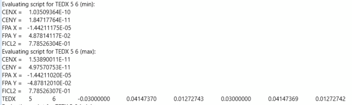
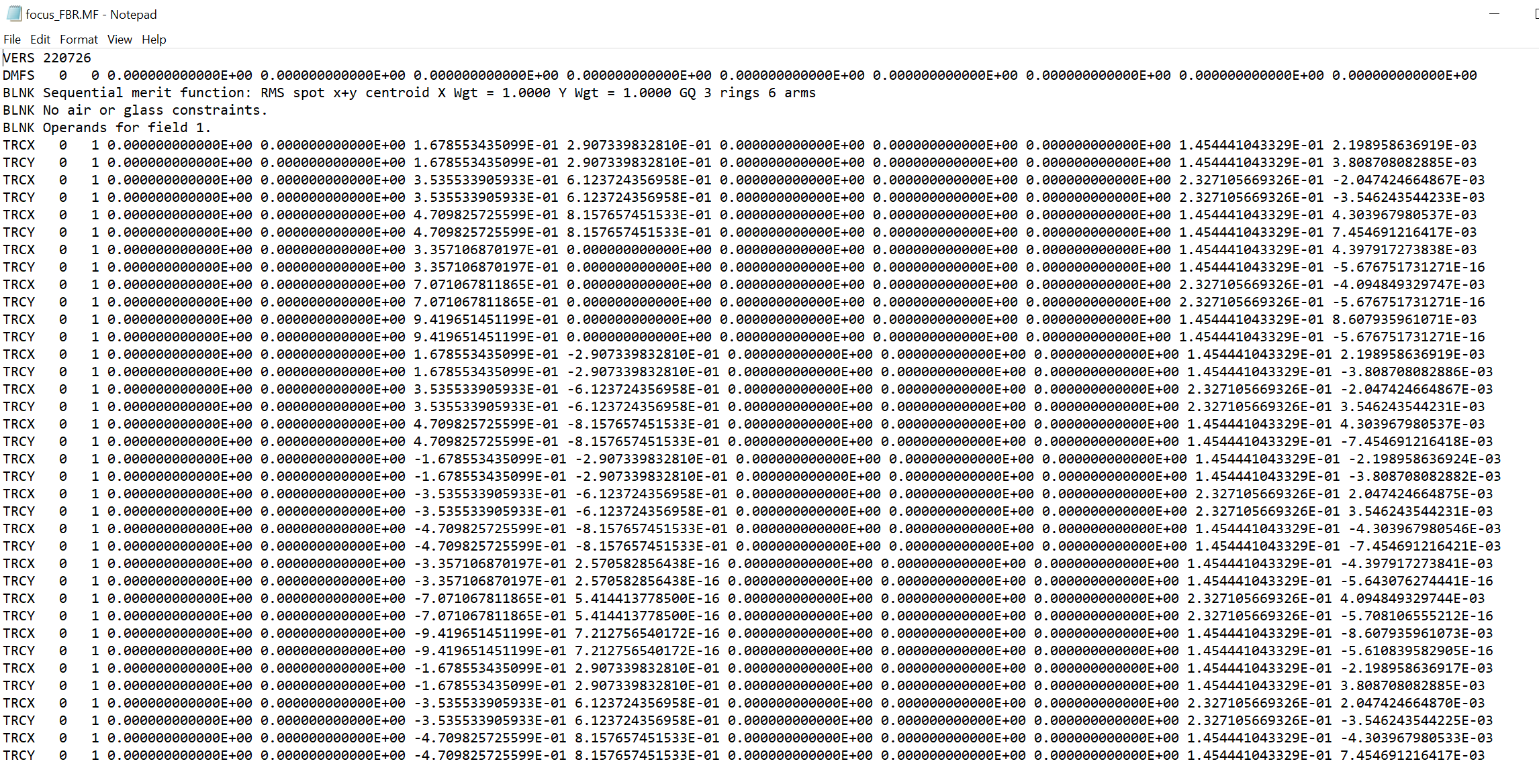
To verify the results, I let Zemax save a file for a specific tolerance parameter.
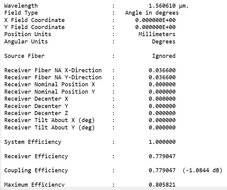
Output of the tolerancing runMerit function for the FICL_14.5.mf part
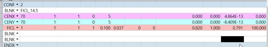
If I compare now the values in the saved file number 10, those values are similar but not equal to the output of the tolerancing run. The FPA values are
compared in my output (-1.442111e-5, 0.04878). Also the fiber coupling efficiency is a little bit off:
compared to FICL=0.778526.
Is there an additional optimization step after my tolerancing script? Where could those differences come from? I am just worried that I still have a fundamental error in there and just get similar values by chance.
I’m glad you are having success, and it’s good that you are carefully checking the results.
First, I would suggest you increase the number of significant digits in your editors; right now you only have three, which really isn’t enough for careful comparison with the tolerance output text data. See Setup → Project Preferences → Editors → Decimals setting.
Second, in your tolerance script you are reporting compensator values mid-way, and then performing another optimization with those compensators, so their final values will not equal the values reported. I suggest you move all REPORT operands to the very end of the script.
Third, the FICL value reported in the tolerance results text window should be identical to that in the merit function of your *saved* file (the one generated using the SAVE tolerance operand). Whether or not this value agrees with the separate stand-alone fiber coupling analysis depends on the settings you use for this stand-alone analysis (sampling resolution, Huygens (yes/no?), align to chief ray?, etc.). I don’t know what settings you used, so I can’t say why the values are slightly different. I can say that if the analysis window settings match those of the FICL merit function operand, the coupling efficiency will be exactly the same for the two.
Fourth, I suggest you consider a higher sampling resolution for the FICL operand, say 3 (128 x128), or perhaps 4 (256 x256) or more depending on how much spatial wavefront aberration you have in the exit pupil. The usual test is to keep increasing the resolution until further increases don’t make a meaningful difference. In other words, you want adequate resolution for the problem at hand, but no more than that since excess resolution will only slow down the calculation without providing any benefit.
Lastly, for your final optimization in the tolerance script, you may want to bump up the number of cycles to say 10. You have three compensators for this last step. When you combine the (x,y) beam steering with the fiber z-axis translation, you may likely need to allow the optimization to run longer. I typically separate the transverse (x,y) compensation from the longitudinal (z) compensation, because the corresponding two optimizations are numerically less demanding, but what you are doing is fine, just make sure the optimization runs long enough to stabilize.
@Markus could you please share your merit functions (focal plane*.mf, xy*.mf) as I tried to replicate your ones without any luck. The CENX, CENY goes crazy (E+11 values...) resulting in unreasonable limit. My system is just a refractive 2 lens system and a fiber.