Hello all,
I am trying to simulate a Super-Guassian beam n=6 in sequential mode but I am having some trouble. I can't seem to find any way to do it. Does anyone have a suggestion on how I might generate this?
Thank you very much,
Matt

Page 1 / 1
Gaussian Apodization under Aperture in the System Explorer should do what you need. You can set an apodization factor for the Gaussian.
Kind regards,
David
Kind regards,
David
Hi all! Thanks for the question here Matt, and thanks also, David, for providing some feedback!
I just wanted to chime in here to add a bit more information. For one, I don't think the Gaussian Apodization Factor will produce the same distribution as a super-Gaussian. Rather, the Apodization Factor will change the distribution of rays in the pupil with the following equation,
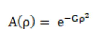
where G is the Apodization Factor and rho is the normalized pupil coordinate. For a super-Gaussian, it can be described by the equation
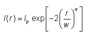
where n is the super-Gaussian factor (equation obtained from https://www.rp-photonics.com/flat_top_beams.html). So, changing the Apodization Factor wouldn't quite be appropriate here.
Currently, there is no direct way to define a beam profile to achieve the super-Gaussian distribution, but there are a couple of workarounds that could be done here:
1) Create a .ZBF file which defines a super-Gaussian beam to use in Physical Optics Propagation (POP)
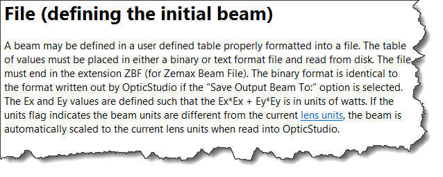
In POP, you have several definitions for your input beam in the Beam Definition tab. One of the Beam Type options is "File," which can take in an arbitrary .ZBF format file. Using either binary or ASCII format, you can define a beam profile which outputs a super-Gaussian distribution--the only limitation here being that this beam is only being used in the POP analysis. You can find some information on defining the .ZBF in our Help Files at "The Analyze Tab (sequential ui mode) > Laser and Fibers Group > About Physical Optics Propagation > Defining the Initial Beam > File (defining the initial beam)":
2) Create a User Defined Surface (UDS) with the transmittance to create a super-Gaussian distribution
This approach is certainly more work to take on, but with the correct implementation, you could create a UDS with a radial transmittance definition to create the super-Gaussian shape you'd like. This way will require writing some C\C++ code and compiling it into a .DLL for use with the UDS, but with this approach, you'd be able to use all the ray-trace analyses rather than just using POP, if that is what suits your needs. For more information, you can take a look in the Help Files at "The Setup Tab > Editors Group (Setup Tab) > Lens Data Editor > Sequential Surfaces (lens data editor) > User Defined" as well as our provided sample code files for different surface types (the default file path for the source .C files is "C:\ ... \Zemax\DLL\Surfaces"). There is also a Knowledgebase article called "How to compile a User-Defined surface" which walks through compiling your code into a .DLL.
Of the two methods, the most straight-forward one is, in my opinion, creating a .ZBF file for use in POP. The trade-off there would then be using only POP for that distribution, but depending on your analysis needs, you might be using that tool anyway.
Feel free to add any any details here if you think I've missed something!
Thanks, Angel.You’re right. I stand corrected! :-)
Could the Slide object provide a (pixelated) workaround?
Hey Davy, thanks for the input! Yes, the Slide Surface would basically be the same thing as creating a UDS with a defined transmission. As you've noted, the limiting factor there is the resolution of the bitmap file you're using with the Slide Surface.
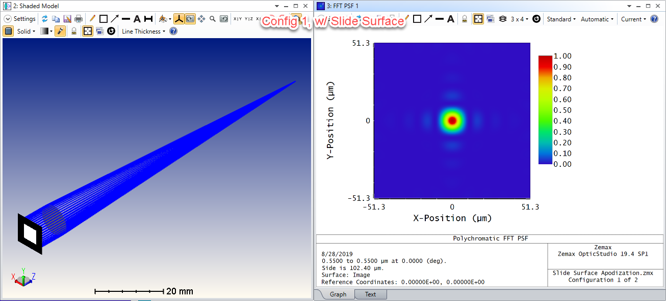
I thought I'd play around with a simple system that uses the Slide to demonstrate how one might go about doing this. In the simple system, I have two configuratons:
As expected, we can see a difference in our results for ray tracing between the two configs--for example, the PSF shows how our focus spot changes between the two distributions.
In case anyone was interested, I've also attached the archive of this file as "Slide Surface Apodization.ZAR".
The only note I should make here about this approach, as well as the UDS, is that the transmission you've defined with either method will affect your final results when looking at efficiency. This is simply a result of the fact that the built-in apodization accounts for the total energy entering the system even when you've changed it to something like Gaussian. When you apply a UDS or the Slide Surface, you are filtering out rays which have already been generated. For this reason, you will want to see the overall transmission of your UDS or Slide Surface before the rays enter the rest of your optical system so that you have the proper baseline to compare to when evaluating system efficiency.
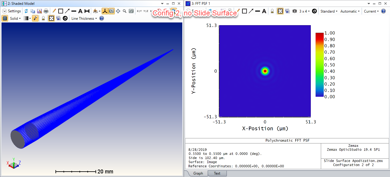
I thought I'd play around with a simple system that uses the Slide to demonstrate how one might go about doing this. In the simple system, I have two configuratons:
- Config 1: A single, on-axis beam passes through my Stop surface with the Slide object co-located (this is to ensure that I am changing the "distribution"/intensity of rays in pupil space), a Paraxial Lens focuses the now-apodized beam (shaped based on the 'square.bmp' file)
- Config 2: The Slide Surface is ignored, and is replaced by a dummy surface with the same thickness as the Slide Surface
As expected, we can see a difference in our results for ray tracing between the two configs--for example, the PSF shows how our focus spot changes between the two distributions.
In case anyone was interested, I've also attached the archive of this file as "Slide Surface Apodization.ZAR".
The only note I should make here about this approach, as well as the UDS, is that the transmission you've defined with either method will affect your final results when looking at efficiency. This is simply a result of the fact that the built-in apodization accounts for the total energy entering the system even when you've changed it to something like Gaussian. When you apply a UDS or the Slide Surface, you are filtering out rays which have already been generated. For this reason, you will want to see the overall transmission of your UDS or Slide Surface before the rays enter the rest of your optical system so that you have the proper baseline to compare to when evaluating system efficiency.
Enter your E-mail address. We'll send you an e-mail with instructions to reset your password.
Need more help?
To Chinese users:
Do not provide any information or data that is restricted by applicable law, including by the People’s Republic of China’s Cybersecurity and Data Security Laws ( e.g., Important Data, National Core Data, etc.).
不要提供任何受适用法律,包括中华人民共和国的网络安全和数据安全法限制的信息或数据(如重要数据、国家核心数据等)。