I am a graduate who has only just started using non-sequential Zemax in the last few weeks and now I am moving on to using sequential Zemax. I am hoping to gain a little bit of guidance on how to make the model that I need.
I am modelling a collimated beam upon a cylindrical lens and looking at the line of spots created in the image plane. I am hoping to analyse the spot size and distortion created in the image plane as I vary the tilt and height of the field on the lens. Some guidance on how best to do this in sequential Zemax would be great.
Best answer by David
Hi Eleanor,
Since you want to model a collimated beam, you likely want a single field in angle space with an angle of 0 degrees. To collimate the beam, the object is at infinity. The beam width can be defined by setting the aperture to Entrance Pupil Diameter.
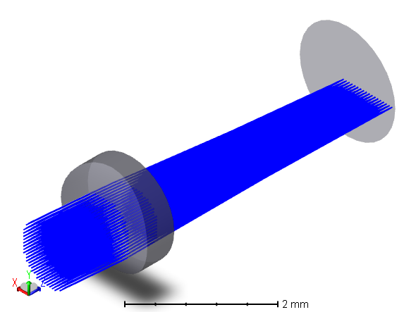
A cylindrical lens can be made using a Biconic or Toroidal surface followed by a standard surface. The lens will of course focus in one plane only and when focused on the image plane produce a spot in the form of a line.
For optimization, the Optimization Wizard can be used to construct a merit function targeting an RMS spot size of zero, with either X Weight or Y Weight set to a weight of 1 depending on the orientation of the lens, and with the other at a weight of 0.
To shift or tilt the beam on the lens, a Coordinate Break can be placed before the lens and used to shift and/or tilt everything after the break, which is equivalent to tilting the beam. The semidiameter of the lens should be fixed so that the lens diameter does not change when the beam is changed.
A standard spot diagram can display the spot, which will be a line.
Since you want to model a collimated beam, you likely want a single field in angle space with an angle of 0 degrees. To collimate the beam, the object is at infinity. The beam width can be defined by setting the aperture to Entrance Pupil Diameter.
A cylindrical lens can be made using a Biconic or Toroidal surface followed by a standard surface. The lens will of course focus in one plane only and when focused on the image plane produce a spot in the form of a line.
For optimization, the Optimization Wizard can be used to construct a merit function targeting an RMS spot size of zero, with either X Weight or Y Weight set to a weight of 1 depending on the orientation of the lens, and with the other at a weight of 0.
To shift or tilt the beam on the lens, a Coordinate Break can be placed before the lens and used to shift and/or tilt everything after the break, which is equivalent to tilting the beam. The semidiameter of the lens should be fixed so that the lens diameter does not change when the beam is changed.
A standard spot diagram can display the spot, which will be a line.
Thank you for your reply. That information was really helpful, thanks.
Now that I have got the model set up, I am wondering how I can analyse the spot size in the image plane.
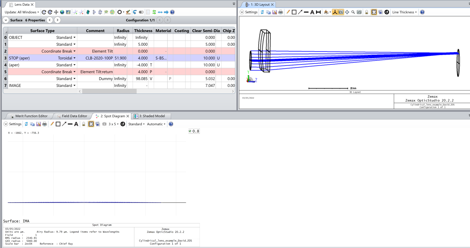
This is my model so far:
I can see the RMS radius here is about 2.5mm (bottom left corner). Seeing as my image is a line, what would be the best way to extract a similar parameter to RMS radius of the spot size in x and y for the line?
The merit function design I mention is able to optimize for spot size on only one axis, but I do not know of a merit function operand or analysis tool that reports spot size for a single axis directly. In non-sequential mode there are operands to report spot RMS on a given axis. Sequential mode merit function operands for spot size, like RSCE, report the size of the 2D spot.
The X & Y rms spot sizes can be fairly easily computed in the merit function by using the wizard to generate the X and Y spot operands (TRAX and TRAY aberration operands) using the weight parameters as described above by David, in combination with a few extra operands to form the spot sizes.
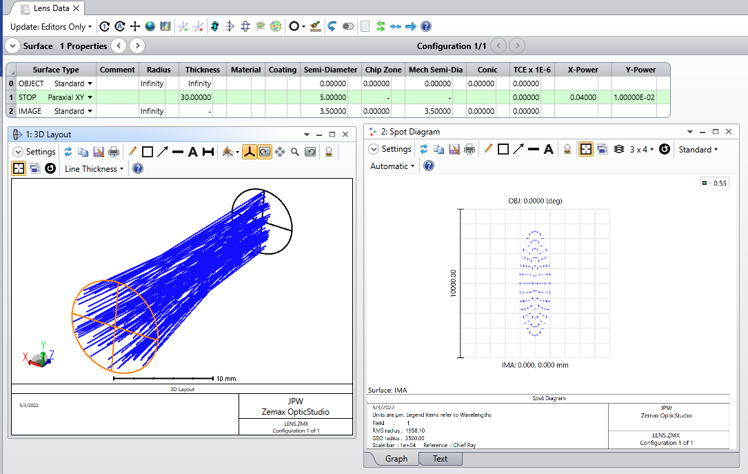
Here’s a simple example using a ParaxialXY lens.
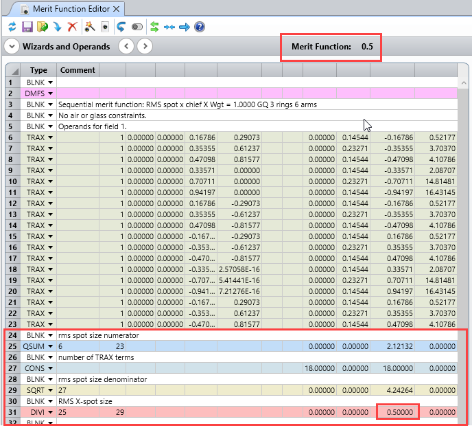
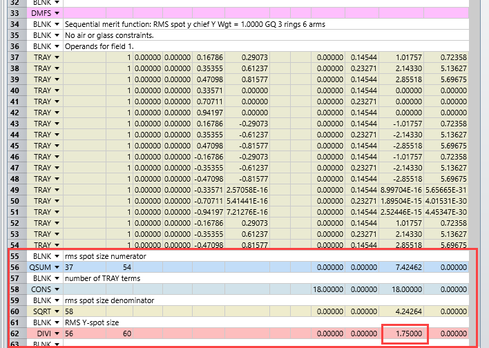
First, use the MF wizard to generate the spot size with X-Weight = 1 and Y-Weight = 0, then find the rms X spot size by computing the RSS of the TRAX operands and dividing by the square root of the number of TRAX terms:
Note: If all we wanted was the X rms spot size, we don’t even need the extra operands, the default merit function will itself evaluate to the correct value. However, if we want both X and Y spot sizes then the extra operands above can be added.
Next, for the Y rms spot size, go back to the MF wizard and repeat using X-Weight = 0 and Y-Weight = 1, but be sure to insert this default set of TRAY operands *after* the existing X terms. Then, add the same set of extra operands to compute the Y rms spot size:
I like to calculate such parameters manually, too - sometimes one just want to be sure how certain values are calculated or extracted by the software :)
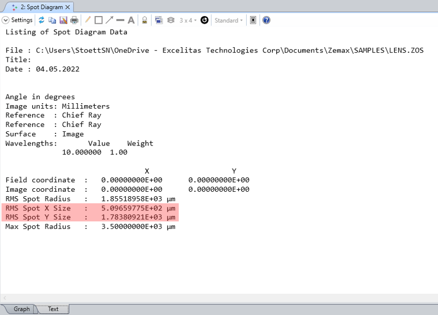
But you can receive the individual x and y components of the rms-value from the spot diagram analyse tool. If you switch from graph to text, you’ll also see the values.
In reply to Jeff’s comment: I seemed to have recreated what you have done somewhat but I have a few questions.
Firstly, please could you explain the thought behind the calculation for the spot size? I am assuming that the method proposed involving the merit function editor should give the same result as the values defined in the Text tab proposed by Sven?
Also, it seems my Zemax model automatically defaults to the operands TRCX and TRCY instead of TRAX and TRAY. Could you explain the difference between these and is the difference significant? How would I go about using TRAX instead of TRCX? I can only seem to change each individual cell manually.
@Eleanor: The rms value of any discrete set of numbers is,
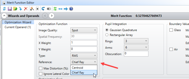
In our case, for the x spot size, the values are simply the x-coordinates of the ray intercepts with the image plane (i.e., the transverse ray aberration values taken along the x-direction), measured either with respect to: (1) the central chief ray, in which case the x values are synonymous with the TRAX terms, or (2) the spot centroid, in which case the x intercept values are given by the TRCX terms. The choice between these two options is available in the Merit Function Wizard:
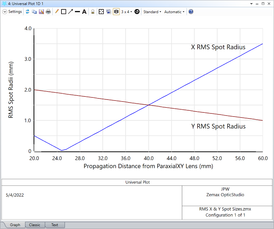
Now with regard to the rms values reported in the Spot Diagram Text output, there are a few key differences compared to the Merit Function approach. First, the ray patterns in the Spot Diagram are different from those available in the Merit Function Wizard. As a consequence, the two approaches will not yield the exact same values. In the MF Wizard, I almost always use the Gaussian Quadrature pattern, which is a very efficient way to sample the pupil. Even if a “Square” ray pattern is selected for both schemes, it appears as though there is a shift between the two patterns (the Spot Diagram includes the central chief ray, while the MF Wizard does not because the sampling options are always even, such as 4x4, 6x6, etc.). Second, when using the MF approach, it is easier to access the spot size values, say for use in a Universal Plot, a ZPL script, or an optimization involving both spot sizes simultaneously. Here is an example of a Universal Plot showing the change in the x and y rms spot radii as a function of distance from the ParaxialXY lens: