Solved

High NA system design - Collimated beam

  • September 26, 2024
  • 9 replies
  • 556 views

CJ27
  • Visible
  • 24 replies

Hi there friends from the OpticStudio community,

Today I have a question related to a general optics design problem.

I’m trying to generate a system similar to what is presented in the following publication:

https://opg.optica.org/ol/fulltext.cfm?uri=ol-42-6-1043&id=360492

In essence, the design problem consists of generating a high NA system which can be used to image molecules or atoms in a vacuum environment. 

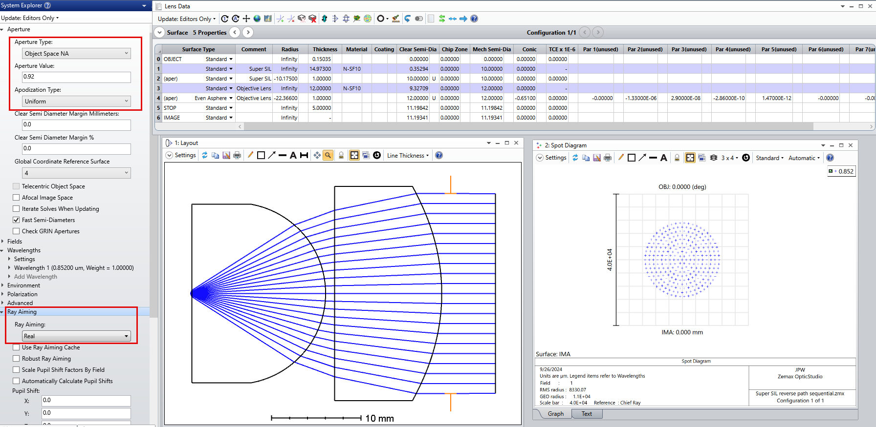
The approach used in this case consists of using a Weierstrass type solid immersion lens in combination with two aspherical surfaces in order to generate a collimated beam for an on axis point object.

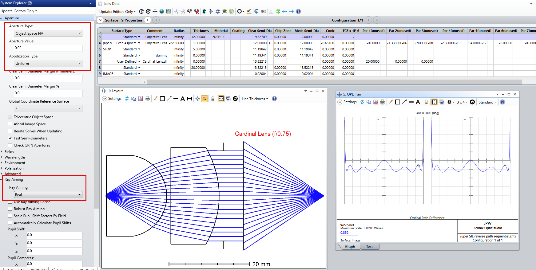
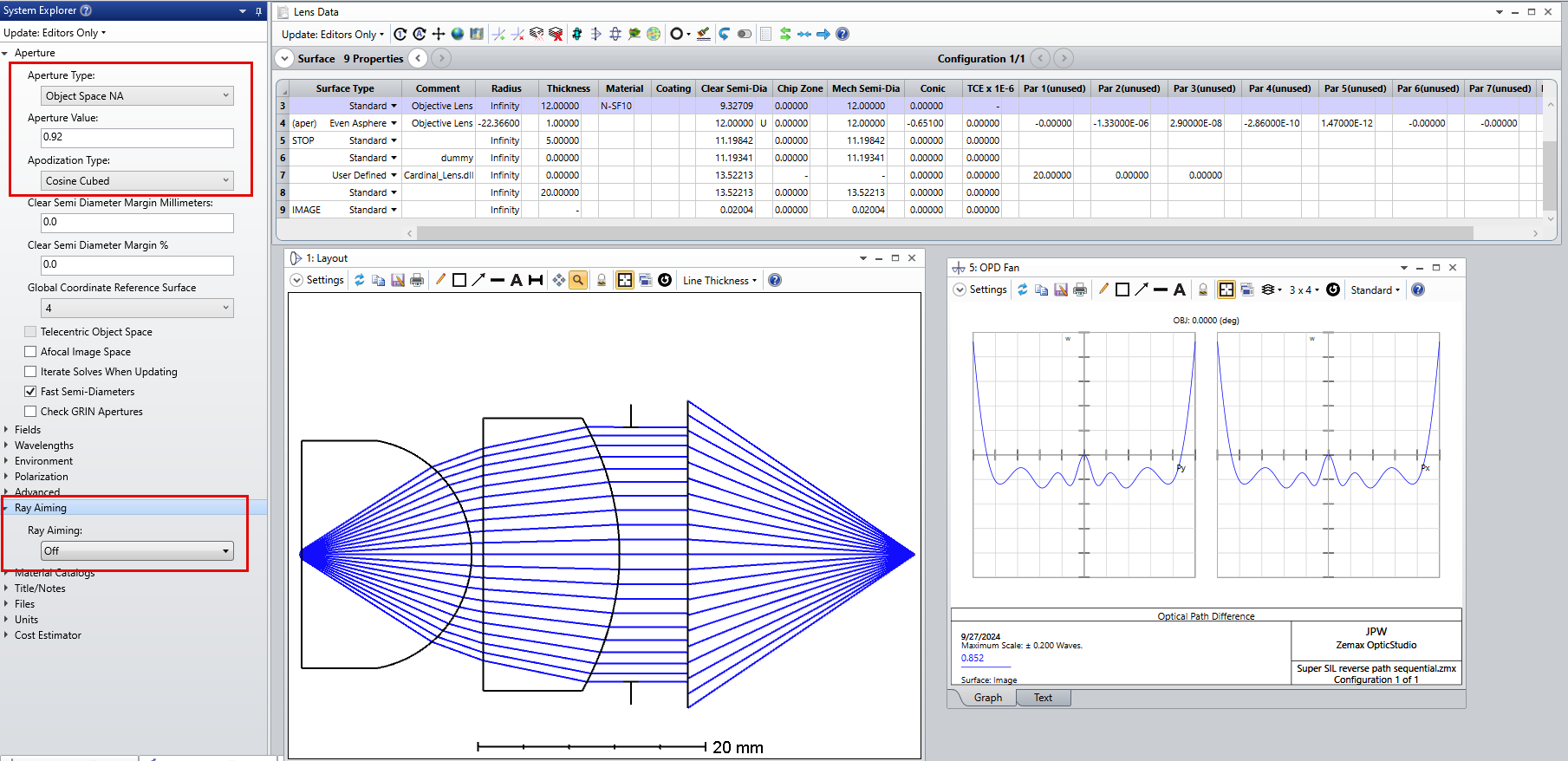
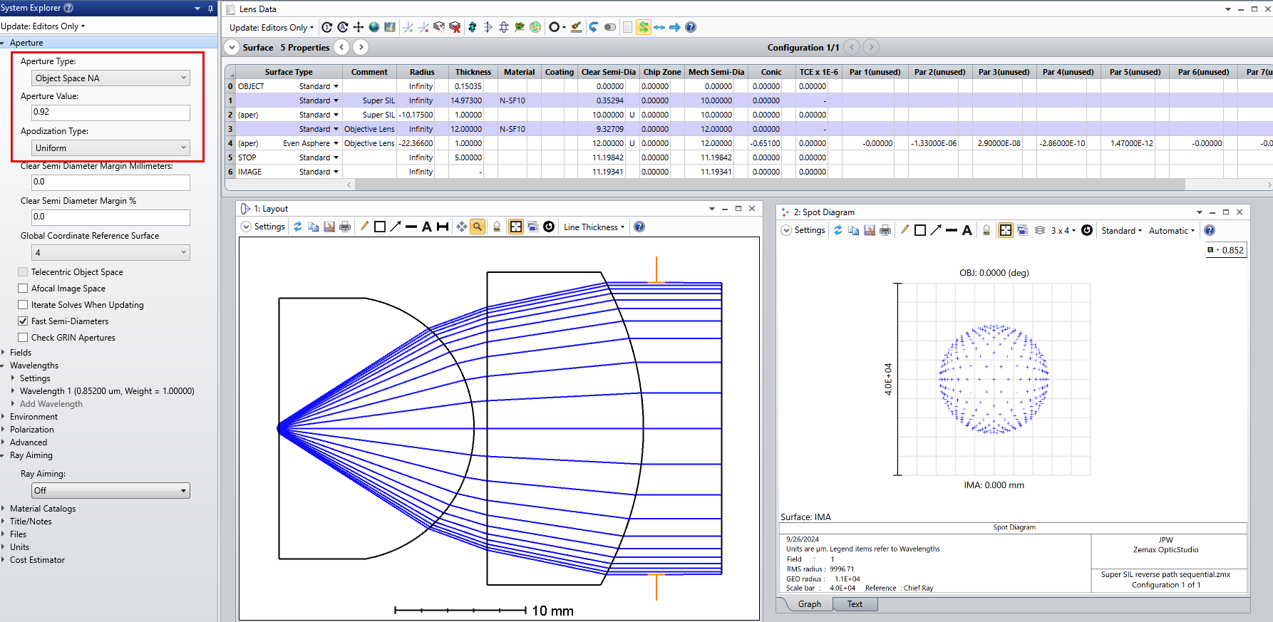
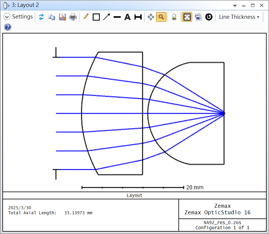
Since the geometry of the Weierstrass geometry is fixed, the only degrees of freedom that I have are the parameters related to my two aspherical surfaces. In the following figure you can take a look to the system I have at the moment:

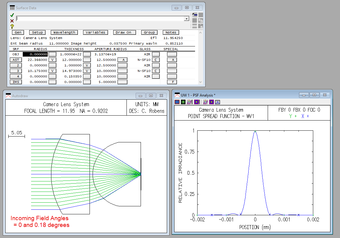
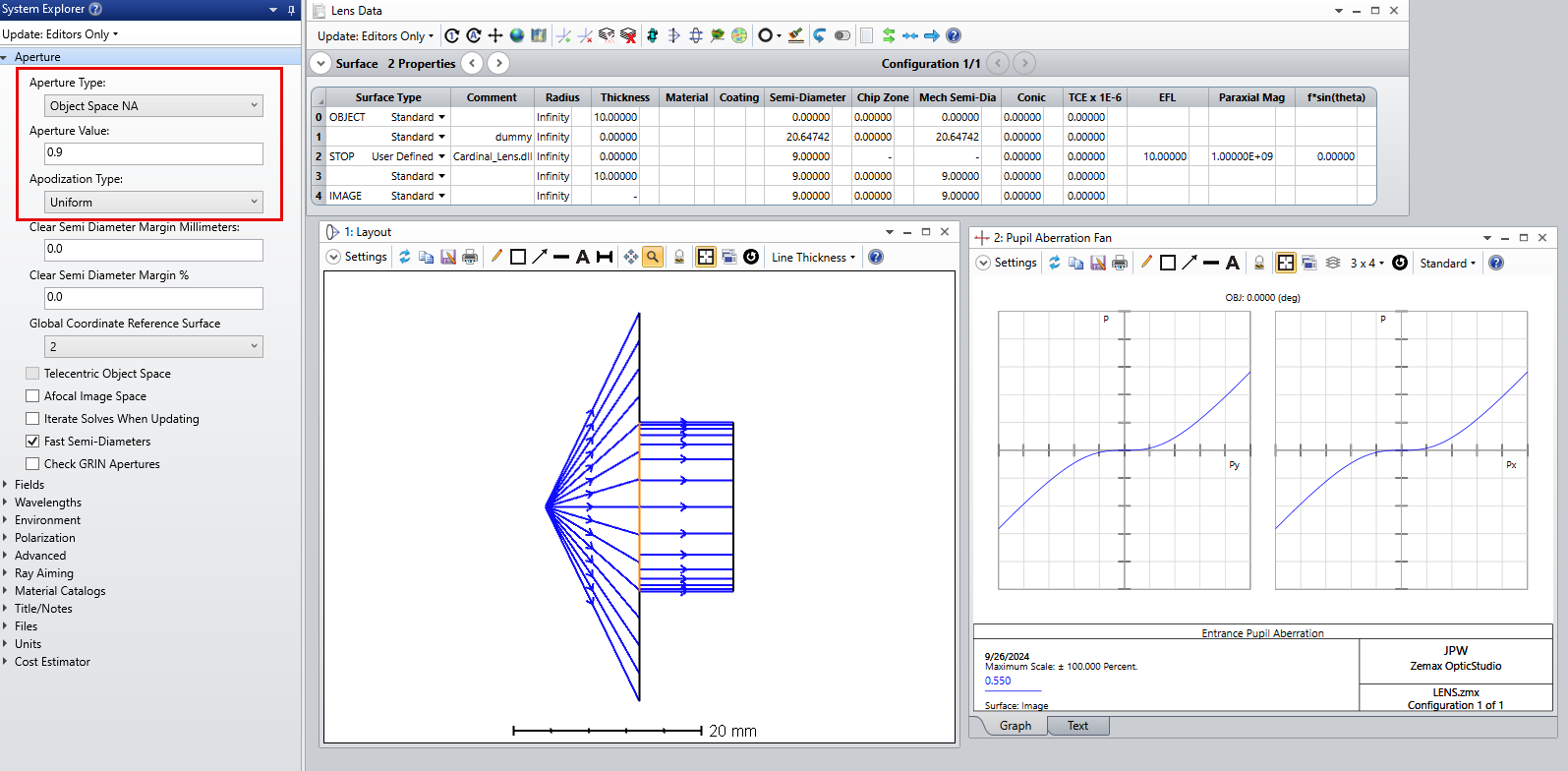
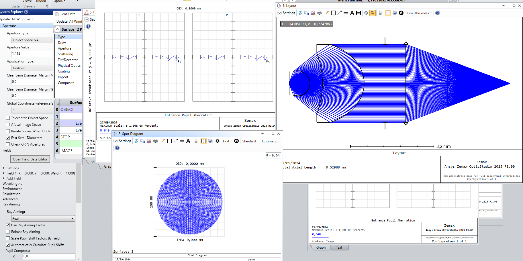
In this case, I optimized this system in the afocal configuration with the merit function defined to have a well corrected planar wavefront. After that I added the paraxial lens just to evaluat the PSF and to see how well corrected my system was.

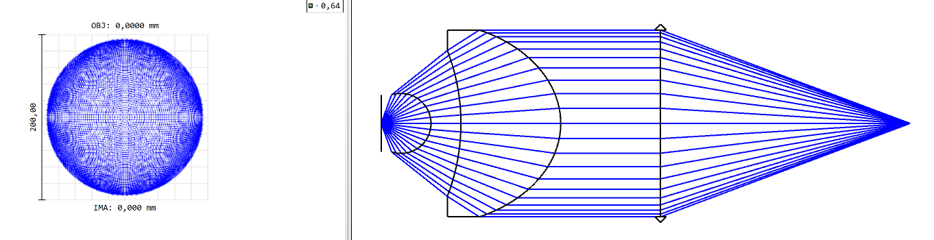
From the PSF evaluation I get a Strehl ratio of 1.0 and also from the wavefront map I get a well corrected performance.

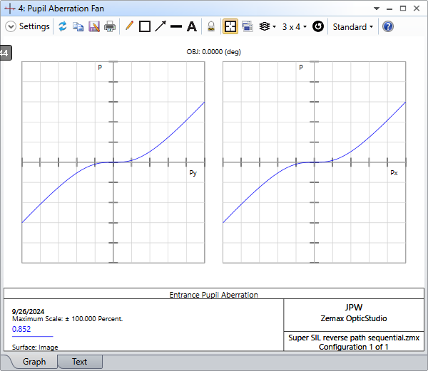
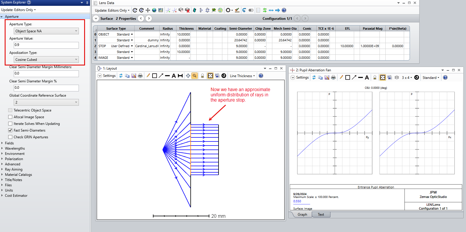
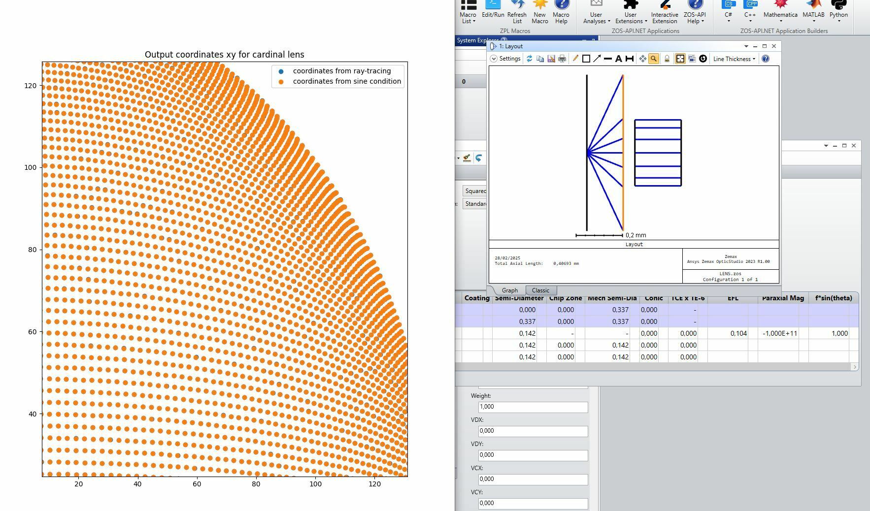
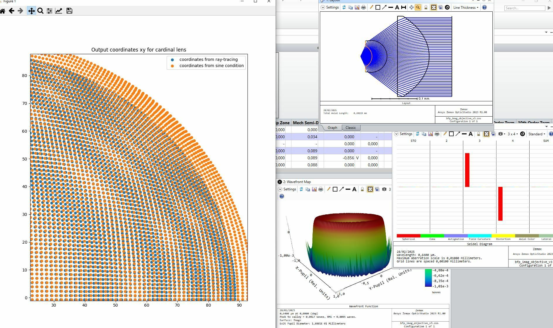
However, if you observe the ray density distribution right after the second aspherical surface and also from the spot diagram on the left side of the optical system, you can clearly see that the rays are not evenly distributed in the “collimated space”.

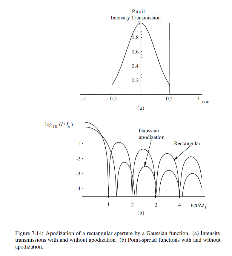
From what I know, if I had a uniform illumination right in front of the paraxial lens (given that the wavefront is well corrected) I would then get an ideal airy disk at the focal plane.

However, from such non-uniform ray density, I get an airy pattern that has stronger side lobes in contrast to the “ideal airy disk” case. 

Having said this, my question is then the following: If I wanted to generate an ideal imaging system, should I also care for the ray density distribution in the collimated set of rays? Is this something that is considered while doing these type of optical designs? If yes, how can I impose this condition into the optimization routine? 

All comments and feedback will be highly appreciated! 

Best answer by Jeff.Wilde

@CJ27

I think the way you originally optimized the lens system via afocal mode with wavefront error minimization is fine.  In that case I don’t think it matters whether or not you have ray aiming turned on because the OPD calculation is done over the entire pupil based on the user-supplied sampling -- as long as the sampling is sufficient, the OPD function should be independent of the ray apodization (or the ray uniformity in collimated space). 

However, I would not suggest optimizing with the paraxial lens in place unless it is operating at f/4 or slower.  As noted in the help documentation, the OPD calculation for a paraxial lens is prone to error if the f/# is too low.


If you did want to include a perfect thin lens at low f/#, here are examples of doing that with the Cardinal Lens.  The Cardinal Lens, if used properly, will compute the correct OPD for low f-numbers.  Information on how to use the Cardinal Lens is provided in Section 4 of this paper Ray-tracing model of a perfect lens.  It works a little differently than a paraxial lens surface; one main difference is that the thickness parameter of the Cardinal Lens surface corresponds to the separation between the principal planes of the lens (i.e., the Cardinal Lens can mimic an ideal thick lens, but if the surface thickness is set to zero then it’s an ideal thin lens).

Case 1 (uniform apodization with real ray aiming)


Case 2 (cosine-cubed apodization without ray aiming)


In both cases you see the OPD fans (wavefront error functions) are quite similar, with the differences being well below the diffraction limit. 

Lastly, I’ll mention that lens design is often done in the reverse direction, going from collimated object space to focused image space.  That’s how the authors of the paper did their design (in  OSLO):


In this case, you don’t have to worry about ray aiming because the entrance pupil (EP) corresponds to the aperture stop (AS).  So uniform apodization will obviously fill both the EP and the AS uniformly.  You would most likely want to change the aperture type to Entrance Pupil Diameter and make sure your field points are defined in terms of angles. 

Regards,

Jeff

View original
Did this topic help you find an answer to your question?

9 replies

Jeff.Wilde
Luminary
Forum|alt.badge.img+3
  • Luminary
  • 491 replies
  • September 26, 2024

@CJ27 

Try using cosine-cubed apodization,


That should help improve the uniformity in collimated space.  The PSF will change depending on the ray distribution because that, in turn, corresponds to a change in the exit pupil apodization.  For more detail, see Goodman’s book on Fourier Optics (Sec. 7.4.5, “Apodization and Its Effects on Frequency Response”).  Here’s an example of uniform vs Gaussian apodization:


Regards,

Jeff


Jeff.Wilde
Luminary
Forum|alt.badge.img+3
  • Luminary
  • 491 replies
  • September 27, 2024

I was giving a bit more thought to this problem and have some additional thoughts.  I took a look at the referenced paper, and it appears the “Weierstrass” solid immersion lens is better known in the optical data storage world as a “Super SIL” (versus a standard SIL that is a simple hemisphere). 

Using the layout details provided in the paper’s supplement, the non-uniform ray distribution in collimated space is indeed readily observed with the aperture stop placed at the objective lens and the aperture type chosen to be Object Space NA with Uniform apodization.

In this case, the paraxial entrance pupil is located about 33 mm away from the object plane and the source ray distribution is chosen to uniformly fill this pupil.  However, an actual point source radiating uniformly in angle space would produce a cosine-cubed power distribution on the flat entrance pupil plane.  Here’s a good article that mentions this detail:  What does the term apodization mean?

In this high-NA collimation system, there is significant pupil aberration:

which in turn means that even though the paraxial entrance pupil may have a uniform distribution of rays, by the time the rays reach the aperture stop the ray distribution is very non-uniform.  This is because there is not a simple linear mapping between the paraxial entrance pupil and the stop (recall the paraxial entrance pupil is simply a paraxial image of the aperture stop, but in reality there is substantial distortion present). This is to be expected and has nothing to due with conventional lens aberrations.  In fact, the same behavior can be found by using a “perfect thin lens” that obeys the sine condition (not a paraxial lens that is far from correct when used as a high-NA collimator).  Here is an example:


It is based on the Cardinal Lens user-defined surface, which models a perfect lens.  See the following link for more detail:


In any event, the problem is corrected by using cosine-cubed apodization:

In this case the rays do not have a perfect uniform distribution, but they are close to uniform.

However, another solution comes from keeping uniform apodization in place, but turning on real ray aiming.  So, in the Super SIL case it looks like this:

Now the ray distribution at the aperture stop in collimated space is truly uniform. 

Which approach is best?  I think the cosine-cubed version may be the more physically accurate choice for a real point source object like a fluorescing molecule, but ultimately I suppose it is up to the user to decide.

Sorry for the rambling explanation, but it’s actually a very interesting problem.

Regards,

Jeff


CJ27
  • Author
  • Visible
  • 24 replies
  • September 27, 2024

Hi @Jeff.Wilde,

Thanks a lot for the really nice reply and feedback. A lot of helpful information was given there 😀

In my original design (which is not the same as from the paper. The paper I use it as a reference for a high NA imaging objective based on the Weierstrass geometry) I had used an aperture of type “Object cone angle” with the aperture stop set directly at the Weierstrass surface.

After changing the aperture stop type to “Object space NA” and setting the STOP surface right after the second aspheric surface as you did, and finally using real ray aiming I can now see that I obtain a uniform distribution of rays in the collimated space:


Clearly, the pupil aberrations are significantly reduced after using ray aiming and the distribution of rays is also uniform as already mentioned.

In this case, I have not changed any parameter related to the design variables, i.e, I use the same coefficient values obtained from my original optimization which was done without ray-aiming and by using an object cone angle type of aperture.

From this, my question now is: In terms of optimization, what should I care for? Should I care for a uniform ray density in the collimated space and therefore consider the ray aiming option? Or would it be sufficient to just use my original approach without ray aiming and strong pupil aberrations? I dont notice any significant difference in terms of aberrations for the system. The only slight difference is in terms of the PSF, for which in the original case I get a PSF with more significant side lobes than when I have the uniform density (an “ideal” airy disk). I guess that using ray aiming and trying to get rid of the pupil aberrations is something that I would like to consider in general for such a high NA system right? 

Finally, I have tried using your perfect lens DLL model to replace the paraxial lens used to re-focus the collimated beam. However, I was not able to use it successfully. Would it be necessary for this scenario (focusing my colimated beam) to use the perfect lens model instead of the paraxial lens? 

Thanks a lot for the comments and feedback!


Jeff.Wilde
Luminary
Forum|alt.badge.img+3
  • Luminary
  • 491 replies
  • Answer
  • September 28, 2024

@CJ27

I think the way you originally optimized the lens system via afocal mode with wavefront error minimization is fine.  In that case I don’t think it matters whether or not you have ray aiming turned on because the OPD calculation is done over the entire pupil based on the user-supplied sampling -- as long as the sampling is sufficient, the OPD function should be independent of the ray apodization (or the ray uniformity in collimated space). 

However, I would not suggest optimizing with the paraxial lens in place unless it is operating at f/4 or slower.  As noted in the help documentation, the OPD calculation for a paraxial lens is prone to error if the f/# is too low.


If you did want to include a perfect thin lens at low f/#, here are examples of doing that with the Cardinal Lens.  The Cardinal Lens, if used properly, will compute the correct OPD for low f-numbers.  Information on how to use the Cardinal Lens is provided in Section 4 of this paper Ray-tracing model of a perfect lens.  It works a little differently than a paraxial lens surface; one main difference is that the thickness parameter of the Cardinal Lens surface corresponds to the separation between the principal planes of the lens (i.e., the Cardinal Lens can mimic an ideal thick lens, but if the surface thickness is set to zero then it’s an ideal thin lens).

Case 1 (uniform apodization with real ray aiming)


Case 2 (cosine-cubed apodization without ray aiming)


In both cases you see the OPD fans (wavefront error functions) are quite similar, with the differences being well below the diffraction limit. 

Lastly, I’ll mention that lens design is often done in the reverse direction, going from collimated object space to focused image space.  That’s how the authors of the paper did their design (in  OSLO):


In this case, you don’t have to worry about ray aiming because the entrance pupil (EP) corresponds to the aperture stop (AS).  So uniform apodization will obviously fill both the EP and the AS uniformly.  You would most likely want to change the aperture type to Entrance Pupil Diameter and make sure your field points are defined in terms of angles. 

Regards,

Jeff


CJ27
  • Author
  • Visible
  • 24 replies
  • February 28, 2025

Hi there ​@Jeff.Wilde,

Once again, thanks a lot for the provided details with your last reply.

I was going again through your paper on the Cardinal Lens and from there I understood that I can use this model  the behaviour of an ideal Fourier lens. 

In my case, I want to use this Weierstrass based lens system to obtain the fourier space representation of the light emitted by a point source found at the on-axis point in object space.

When using the Cardinal lens with the fsin(theta) flag set to one (for an ideal Fourier lens) and then comparing the coordinates at the back focal plane from the ray-tracing to the coordinates calculated from the explicit use of f*sin(theta), as expected, I can see that the sine condition is satisfied. Here for the explicit evaluation of the sine condition, I have used the front focal length (object space refractive index times the EFL parameter set at the Cardinal lens)


However, once I try to do the same for my Weierstrass lens, well, this is not the same:


For this case, I have taken the EFFL value returned by Zemax which I imagine is not entirely correct here. But even when I “manually” adjust the focal length value so that the coordinates extension are somehow similar, I can see that there is no agreement between the ray-tracing coordinates in the collimated space and the coordinates calculated from the explicit sine condition evaluation.

Would you maybe have some comment on this situation here? Does this mean that my lens design is not close to being an ideal fourier lens system? Would this be related to the fact that the system is not aplanatic? Any suggestion on how could I improve my system design so that I can have better Fourier imaging performance? 

Once again, thanks a lot for the comments and feedback. 


Jeff.Wilde
Luminary
Forum|alt.badge.img+3
  • Luminary
  • 491 replies
  • March 1, 2025

Hi ​@CJ27 

Yes, the Cardinal Lens model supports both an ideal imaging lens with f*tan(theta) distortion and an ideal Fourier lens with f*sin(theta) distortion.  Both versions satisfy the sine condition.  I think you may be confusing f*sin(theta) distortion with the sine condition.  They are separate concepts.  For collimation of an on-axis point, both versions of the Cardinal Lens should yield exactly the same result.  It’s only when you look at off-axis points that a difference occurs.  A lens that is (1) aberration-free (or at least very low aberration) on-axis, and (2) also satisfies the sine condition is considered to be aplanatic.  It will yield low aberration for nearby off-axis points. 

It would appear that your lens may not be aplanatic, so aberrations will arise quickly when moving off-axis due to the presence of linear coma.  An aplanatic lens is free from linear coma.

Now, regarding the ability of your lens to perform an optical Fourier transform, I guess I don’t quite understand what you are trying to do.  Typically, if an object is illuminated with a collimated, normally incident and spatially coherent beam, then the angular content of the light leaving the object is related to the Fourier transform of the object.  However, to observe this, we need to convert the angular spectrum of plane waves into a spatial pattern that we can measure with a pixelated detector.  This is what a FT lens does, it properly maps the incoming angular spectrum into the spatial FT in the back focal plane of the lens. 

In your case, you are working in reverse, going from the spatial domain to the angular domain.  So, I’m not quite sure what you mean when you say you are looking “to obtain the fourier space representation of the light emitted by a point source found at the on-axis point in object space.”  If, instead, what you are trying to do is design an aplanatic lens for use with a point on or nearby the optical axis, then the form of the distortion is not particularly important.  Instead, you basically just want to minimize aberration.  More specifically, you want to try and eliminate spherical and linear coma. You can do that by using two field points, one on-axis and one slightly off-axis, and generating a merit function that seeks to make them both diffraction-limited.  Alternatively, you can use just one on-axis point, then generate a merit function for that point and add the OSCD operand, which will help enforce the sine condition.


Hope this helps…

Jeff


CJ27
  • Author
  • Visible
  • 24 replies
  • March 1, 2025

Hi again ​@Jeff.Wilde,

Thanks for the feedback. I read about this offsense against the sine condition in your paper but I never saw it in Zemax. Thanks for pointing this out here. 

Maybe I can explain a bit more about what I am trying to do. I want to have a design which can be used for doing back focal plane imaging of a point emitter which sits at the on-axis point of my system. (Actually the system is the same as for the original paper I shared at the beginning but here the idea is that instead of using a tube lens to generate a real space image of the atom/emitter I use a lens which images the back focal plane to some camera/detector. In this case, this back focal plane image will have information on the angular spectrum composition of the light being emitted by the point source).


This is something that is done a lot in the field of nanophotonics, actually there is one  review paper in where this imaging technique is explained more in detail:  https://www.degruyter.com/document/doi/10.1515/nanoph-2023-0887/html?lang=en&srsltid=AfmBOorbV-yN2NEaVuhuR6_8INqmIzAJYVLaOPsX6qGOg9Zz4asauI2O


If you take a look to the paper, there it is explained that each plane wave component originating from the point source would be mapped to the back focal plane of an infinity corrected objective and the mapping relationship follows the same expression you provide for the ideal Fourier lens settings : f * sin(theta_inc) 


In fact, when I take a look to your paper, on expressions number 14, this is what I think you were trying to impose there right? That the coordinates in the back focal plane should follow the f*sin(theta_inc) condition, i.e, each incident ray with angle theta_inc is mapped to the back focal plane coordinates x_2,y_2 and the mapping follows the expression given in Eq. 14.

Now if I understand this correctly: this is the condition that needs to be satisfy as close as possible right? That each ray originating from my on axis point is mapped to the back focal plane coordinates according to the sine condition.  Otherwise, there would be no way to map back from the BFP coordinates to ray coordinates (or k vector values) in a “simple” manner right? (i.e, the mapping would not follow such a sine based relationship). 

Another example in where this BFP imaging of point emitters is demonstrated is given in this paper: https://pubs.aip.org/aip/rsi/article/94/6/063703/2897381/Back-focal-plane-imaging-for-light-emission-from-a

Here they use the same idea: A Weierstrass lens based imaging system with an aspheric collector that provides a collimated beam. 

At the end, what my main issue would be is: If the lens that I have do not satisfy the f*sin(theta_inc) mapping from the input rays to the coordinates at the BFP, I cannot interpret the BFP pattern as the k space representation of my point source spectrum right? Only when this condition (which seems to be the same as the Abbe sine condition) is satisfied, then I can think of the BFP pattern as the k space representation of the emitted field by the point source. 

Would this make sense?


Cheng-Mu Tsai

Hi, @Jeff.Wilde, 
I am also interested in this lens design. 
I tried to place long conjugate in object space and short conjugate in image space, that is, reverse design like the example OSLO. 


And I calculated the image space NA, the result shows that it cannot be 0.92. 
From the example OSLO, the image space fno is 11.95425 (EFL)/22 (EPD) = 0.5434
And the image space NA = 0.6771. 
I don’t know what the differences are in these two designs?

Could you please explain why the NA could be different in these two designs?


Jeff.Wilde
Luminary
Forum|alt.badge.img+3
  • Luminary
  • 491 replies
  • March 30, 2025

@Cheng-Mu Tsai,

In Zemax the “Image Space NA” is calculated as the index of image space times the sine of the angle between the paraxial chief and marginal rays, so it is only applicable to low-NA systems.  For high-NA systems, a more meaningful number is the “Working F/#” (or WFNO) because it is calculated using real rays.  Therefore, it’s generally best to use NA = 1/(2 WFNO).  See the help documentation for more detail.

For the lens design published in the paper, when modeled in Zemax, we find WFNO = 0.55305, so NA = 0.904.

OSLO uses different definitions that are based purely on paraxial rays, namely:  WFNO = EFL/EPD and NA = 1/(2 WFNO) = n tan(theta) = n times the axial ray slope.  Here n is the image-space index and theta is the angle of the paraxial marginal ray (which OSLO calls the paraxial “axial” ray).  For the published paper, this yields WFNO = 0.5434 and NA = 0.920.

Personally, I prefer to use the Zemax WFNO and associated NA.

Regards,

Jeff


Reply


Cookie policy

We use cookies to enhance and personalize your experience. If you accept you agree to our full cookie policy. Learn more about our cookies.

 
Cookie settings