
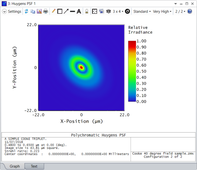
I want to create a universal plot of Huygens PSF FWHM vs wavelength or field.  Is there an operand that would make this possible or do I need to write a script to (or manually) extract the FWHM from the Huygens plot data?  This is for a spectrometer. 

I’d also like to get the local dispersion around a number of central wavelengths.  If you can think of any built-in tools or shortcuts for doing this, please let me know.  Thanks!

@Donna.Waters 


I would do this through the ZOSAPI. Save all the relevant PSFs, either 2D or 3D data. Then I’d use Python and SciPy to fit the PSFs with a 2D or 3D Gaussian (or function of your choice) respectively and extract the FWHM.

You could make an operand as well and in fact ​@Allie did that for non-sequential detectors:

but as you see from her post, there are some assumption about what the PSF should look like and it might be finicky to troubleshoot if your PSFs violate those assumptions. I haven’t tried the operand, but looking at its description if your PSF is not symmetric and its major axis is not aligned with X or Y it might be an issue.

As a side note, if you’re going down the ZOSAPI route, a PSF analysis tools might be a nice contribution to ZOSPy.

I hope this helps and take care,


David


Hello,

computing the FWHM can be quite easier, depending on the precision you need.

Here is a code sample I adapted from a suggested solution found on StackOverflow :

from matplotlib import pyplot as mp
import numpy as np

def peak(x, c):
return np.exp(-np.power(x - c, 2) / 16.0)

def lin_interp(x, y, i, half):
return x[i] + (x[i+1] - x[i]) * ((half - y[i]) / (y[i+1] - y[i]))

def half_max_x(x, y):
half = max(y)/2.0
signs = np.sign(np.add(y, -half))
zero_crossings = (signs[0:-2] != signs[1:-1])
zero_crossings_i = np.where(zero_crossings)[0]
return [lin_interp(x, y, zero_crossings_i[0], half),
lin_interp(x, y, zero_crossings_i[1], half)]

# make some fake data
x=np.linspace(0,20,21)
y=peak(x,10)

# find the two crossing points
hmx = half_max_x(x,y)

# print the answer
fwhm = hmx[1] - hmx[0]
print("FWHM:{:.3f}".format(fwhm))

# a convincing plot
half = max(y)/2.0
mp.plot(x,y)
mp.plot(hmx, [half, half])
mp.show()


@Sebastien G. 


Correct me if I’m wrong but in your code you are also assuming that the FWHM is aligned with one axis of the detector.

In the case of an arbitrary PSF, like the one shown in this article (last Huygens PSF plot):

Then, it would be better to measure the FWHM along a diagonal axis. Hence why I suggested to do a 2D (or even 3D) fit for robustness.

Take care,


David


Hello,

You're right, I'm just so used to work on 1D signals that I didn't think otherwise...


Thanks for your suggestions!  I also found a macro that was helpful for mapping out the spectrum on the detector and generating a plot of the local dispersion.  It’s called Mapping_Function_Resolution.zpl.  It doesn’t give resolution, despite the name, but the dispersion curve is useful.


Reply