I am trying to generate a ray dataset from a data array which represents the Poynting flux at the far-field from a nano-structure which generates a somehow Gaussian-like far-field profile.
This is the process that I used for generating my far-field intensity:
I extract all far-field components (E and H) at a given r distance from my source plane.
Using these far-field components I calculate the Poynting vector components.
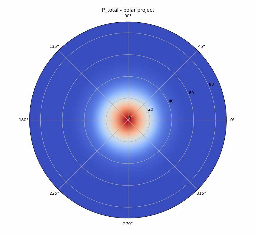
In this case, I have extracted the data over the surface of a half sphere which covers my full upper hemisphere.
This data is extracted from an open source FDTD solver and I know how does the intensity distribution should look like. Below plot shows the computed Poynting flux over the sphere surface projected over a 2D plane. (the radial axis is equivalent to the polar axis and the azimuthal axis represents what it is supposed to)
I have followed Zmx help documentation in order to generate a .DAT file from above intensity information. I generate a file in where each line contains:
0 0 0 m l n flux_from_above
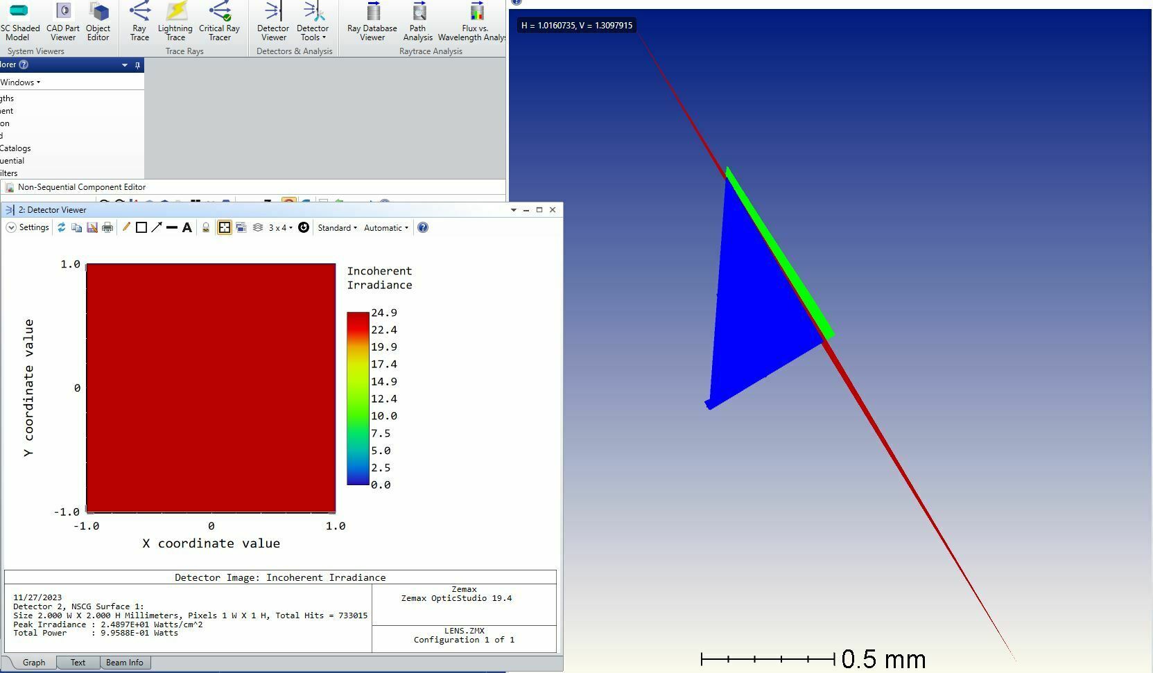
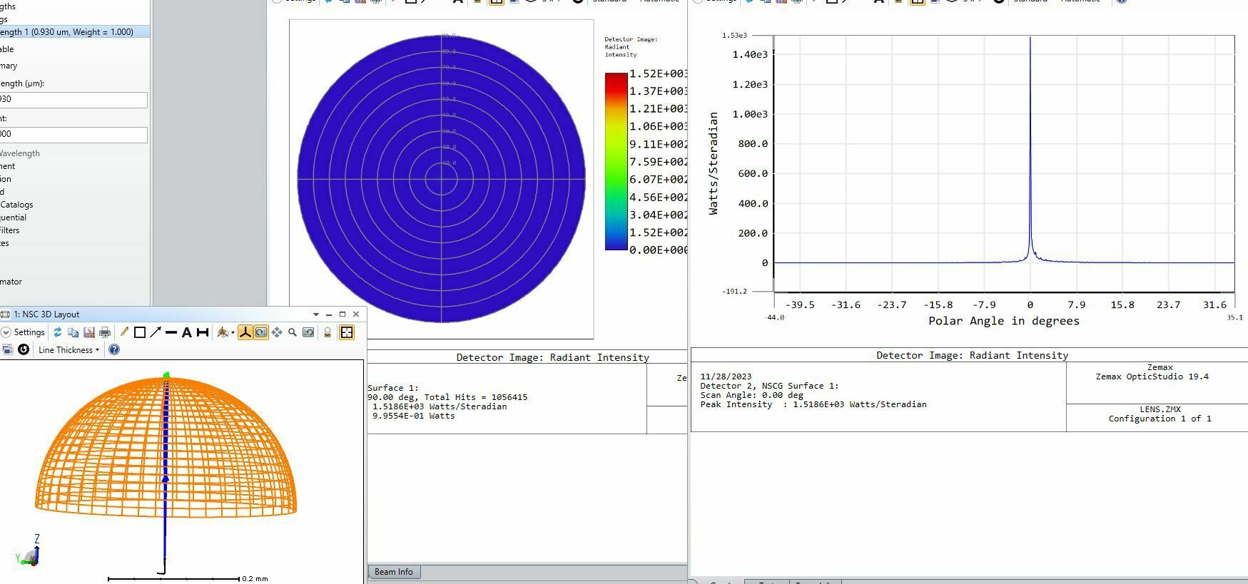
However, once I try to use and import this DAT file into Zmx via a source file, the obtained ray distribution is not what I would expect. Also, by taking a look to the irradiance collected by a detector, I just obtain an uniform irradiance profile:
Additionally, as you might observe, the generated ray distribution does not have the circular distribution shape that I would expect based on the polar plot that I have included above. In fact, the rays are just extending over a line.
Any idea about what could be happening here? Any comment and feedback will be highly appreciated.
Page 1 / 1
Hi there again Zmx community,
I have taken a closer look and I had a problem with the number of pixels used in my detector. By increasing this number I can see that the irradiance on the detector is not uniform. However, I can observe that there is a high irradiance peak at the center of the detector and it is not possible to clearly observe the rest of the structure due to the large contrast in irradiance.
Ideally I would want to obtain a plot similar to the polar plot that I have included above. I have noticed that by if I decrease the size of the detector, the peak irradiance at the center just continues to grow until the point in where I have a single pixel with a really high irradiance and the rest of pixels with 0 irradiance.
Any thoughts or comments on what can be happening here? Any insight and feedback will be highly appreciated!
Change the Detector viewer from “Incoherent Illuminance” to “Luminous Intensity”. That will put you in angle space which is closer to your polar plot. You can also use the “Detector Polar” instead of “Detector Rectangle”
Hi Andrew_Davies,
Thanks a lot for your feedback and help.
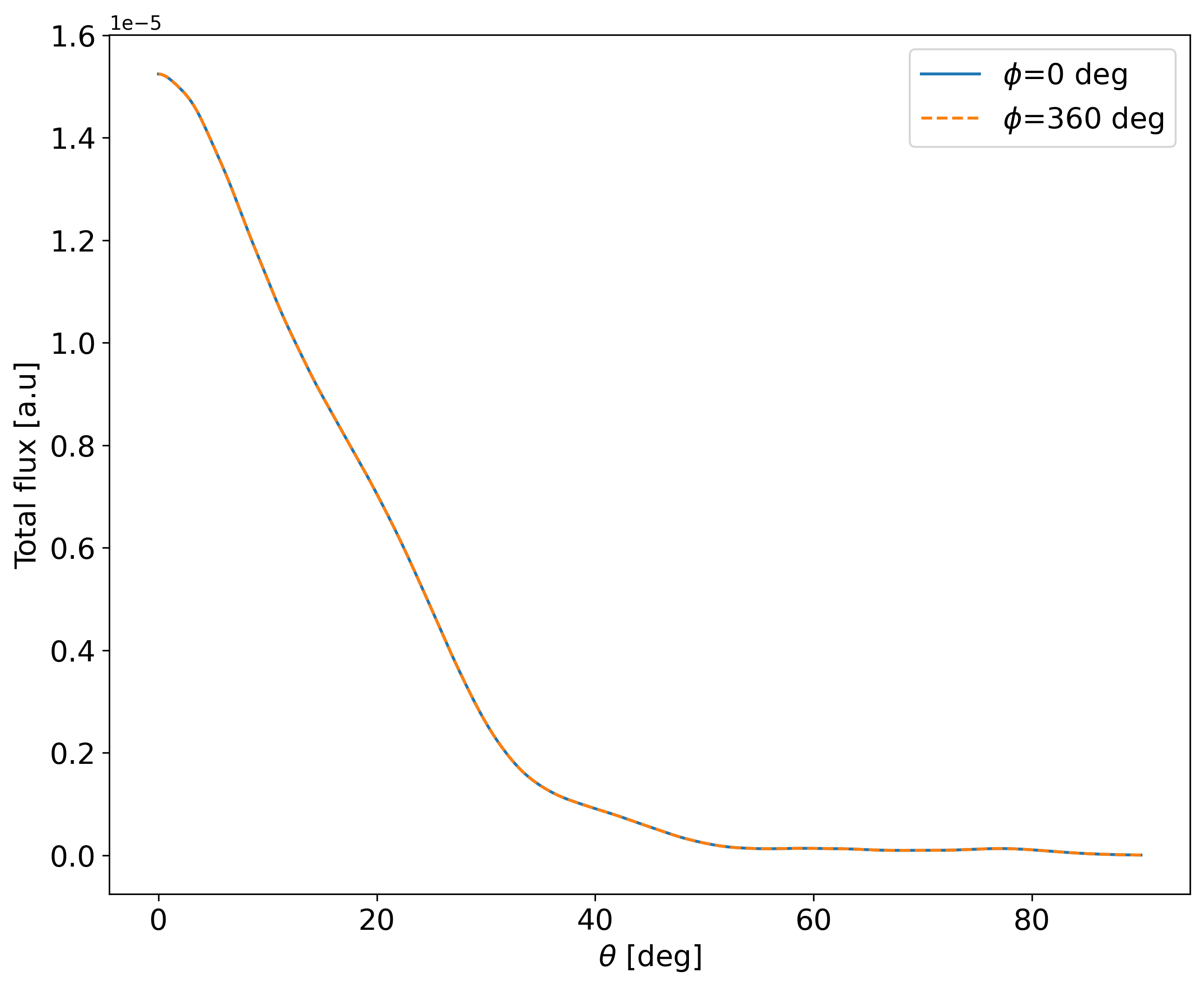
I have tried changing the detector from a “Detector Rectangle” to a “Detector Polar” and restricted the maximum angle to 90 degrees. However, the generated polar plot is not really similar to what I got from my FDTD simulation. Specifically, the extent of my light source in angle space is not well captured in case of this ray-tracing based approach. Below I am showing a cross section of the computed Poynting flux (directly from my FDTD data) as a function of theta (polar angle) for two azimuthal angles (phi=0 and 360)
As you might observe, the flux is supposed to spread over to a maximum polar angle of around 50 degrees. However, in Zmx, this is what I obtain:
In this case, most of the flux is restricted to a polar angle not larger than 10 degrees. What could be going on here? What could I be missing in this case?
I have to say that for my source file data, I just took the computed Poynting flux values directly without any scaling or transformation. As for the direction cosines, this is the way I obtained the values:
l = sin(theta)*cos(phi) / mag(u_vec)
m=sin(theta)*sin(phi) / mag(u_vec)
n = cos(theta) / mag(u_vec)
with mag(u_vec) = sqrt(l**2+m**2+n**2)
Any idea on what could my problem be in this case? Could it might be related to the scaling of the intensity entries that I am using in my source file?
Any comments or feedback will be highly appreciated.
But as a troubleshooting exercise I would try converting your “l m n” direction cosines back into degrees and see if it agrees with what your starting angles. Do this with equations from the Zemax help file to see if there is a convention mismatch. I believe Zemax does it two different ways and I’m not sure which convention is used for the Source file described in Non-sequential Sources helps file “Source File”.
Start by going to the Zemax help file “Detector Rectangle Object” and go to the section “Comments on Detector Rectangle angular binning”. Use these equations to calculate back to degrees and see if it matches your starting point. Then go to the “Field Angles and Heights” help file and use those equations to calculate back to degrees and see if that matches. See if switching conventions solves your problem. Also note that I think both these equations sets are going the Cartesian coordinates in angle so keep that in mind.
Another troubleshooting option is to make a .SDF file with Zemax that is similar to what you want by using the Source Radial to generate rays with a similar angler profile. Then inspect that file and see how the angle look different and try converting it to degrees and see if you get what you expect.
Hi Andrew_Davies,
Thanks a lot for your last reply.
I have given it a closer look and yes you are right, the direction cosines are correct.
I have tried out with a different source configuration:
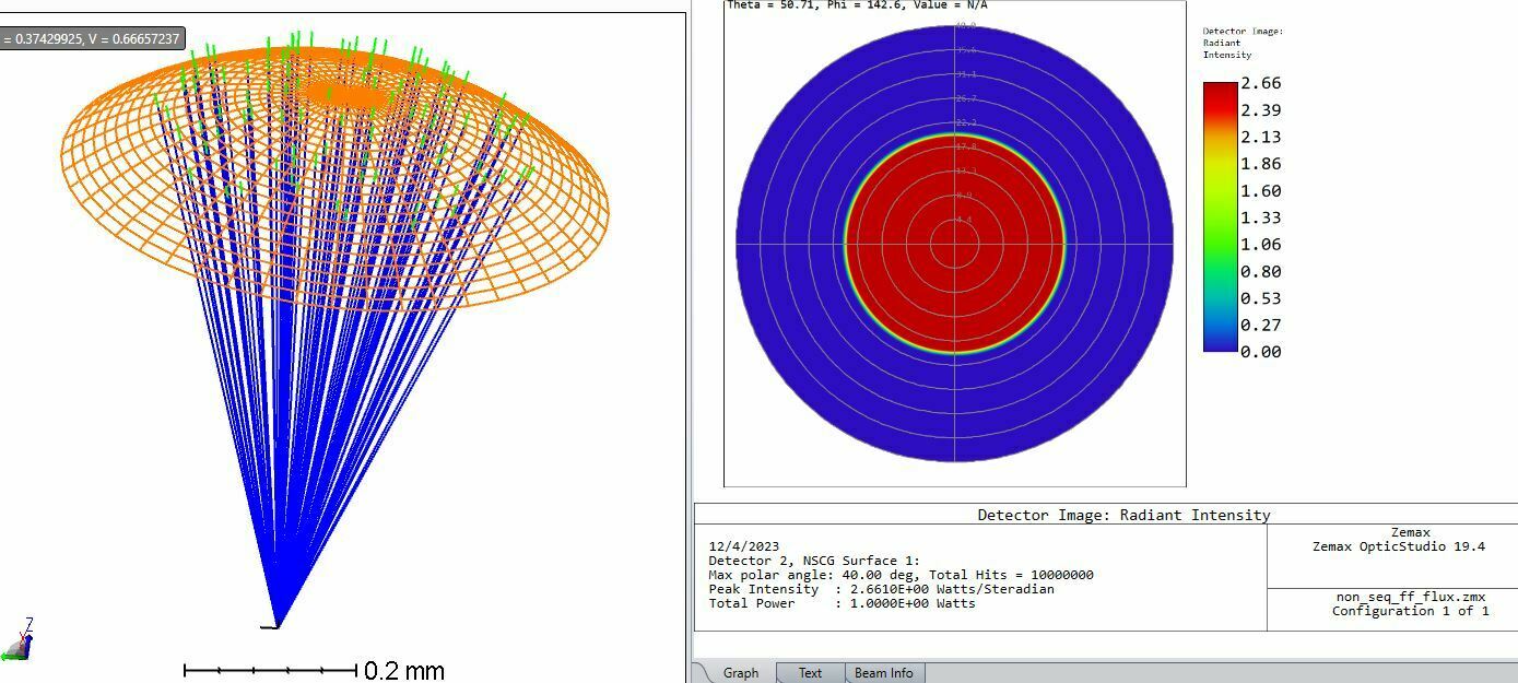
I have defined rays coming from a point (x,y,z = (0,0,0)) defined over the angular extent (theta from 0 to 30 degrees and phi from 0 to 90 degrees) with each ray having an intensity of 1.
If I use this source file in combination with a polar detector, I should observe an uniform intensity profile over the defined angular region right? (Please let me know if my understanding is correct).
However, once I trace the rays from the point source to the defined polar detector, I do not observe a uniform radiant intensity distribution over the defined angular extent.
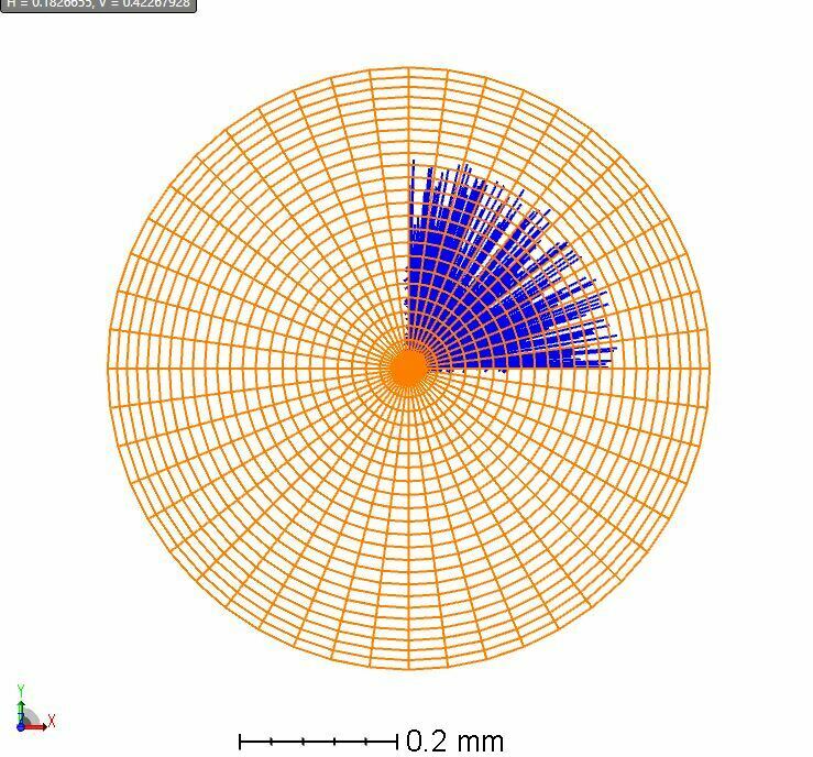
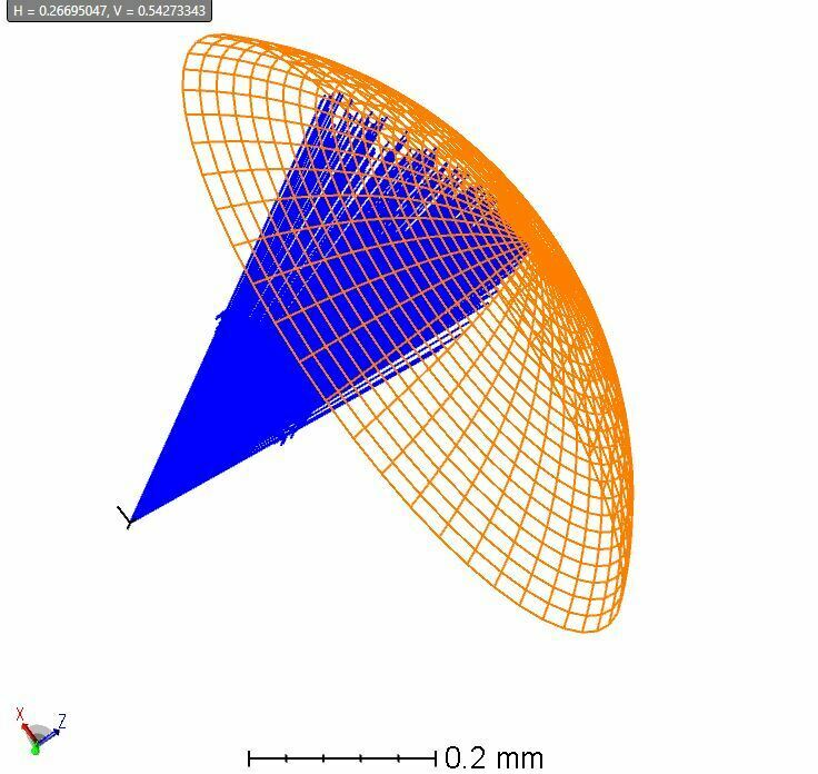
Below you can see a layout with the rays propagating from the source towards my polar detector. You can see that in the phi coordinate, the ray bundle is defined from phi=0 up to phi=90 degrees.
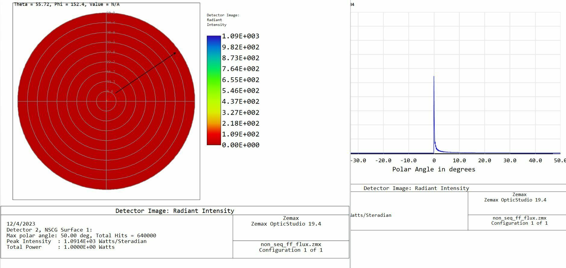
However, as mentioned above, once I do the ray tracing, the projection I get from the polar plot does not show an uniform “energy distribution” as a function of the theta and phi angles.
As you might observe, there is a peak in intensity at the center and then the intensity decreases towards larger theta angles. The distribution is somehow similar along phi.
What do you think about this? What could I be missing here? I would understand that if within the source file I defined the intensity of each ray to be equal to 1, I would then obtain a uniform distribution in angle space right?
Any comments will be welcomed and appreciated.
Hi again Andrew_Davies,
I have found this nice post within Zemax forum that discusses a bit more in detail about polar detectors.
There a native point source with a finite angular extent is used and similarly to what I was mentioning above, the intensity is uniform in angle space. This is what I should get if I define a source file for a point (x,y,z=(0,0,0) and direction cosines (l,m,n) with each ray intensity equal to 1 no?
What do you think?
Below I include an output of a polar detector used in combination with such point source.
I think that the individual ray intensities should be scaled by some factor here I guess. Any idea or reference on how to do this?
CJ27, yes I agree with your expected result. Setting the ray intensity to 1 and emitting them isotopically within the direction cosine range from a point source should make a uniform profile with a sudden transition to zero in the polar detector.
I would try saving the rays you are getting from the native point source into a .DAT file and then examine it in a text editor. See how it’s different from what you have. See if you can recreate it from Matlab/python and import it into Zemax.
Note that the peak in intensity at the center of the polar detector is probably an artifact of the plot. Not from the ray trace . There are some form posts on the issue. It likely comes from the pixels having a very small area at the peak of the polar detector so you can get wide swings in signal at that point form noise.